Jan 1, 2013 - + appears in the sequence XS. + at most once. In fact,. ) ,( k ezz. + appears in XS. + if and only if sk. â¤â¤. 1 and either. X uzk â. + or. X vzk. â+ .
GLOBAL COMMUNICATION ALGORITHMS FOR CAYLEY GRAPHS Vance Faber Big Pine Key, Florida 33043 ABSTRACT We discuss several combinatorial problems that arise when one looks at computational algorithms for highly symmetric networks of processors. More specifically, we are interested in minimal times associated with four communication tasks (defined more precisely below): universal broadcast, every processor has a vector that it wishes to broadcast to all the others; universal accumulation, every processor wishes to receive the sum of all the vectors being sent to it by all the other processors; universal exchange, every processor wishes to exchange a vector with each other processor; and global summation, every processor wants the sum of the vectors in all the processors . §1. Introduction. We discuss several combinatorial problems that arise when one looks at computational algorithms for highly symmetric networks of processors. More specifically, we are interested in minimal times associated with three communication tasks (defined more precisely below): universal broadcast, every processor has a vector that it wishes to broadcast to all the others; universal accumulation, every processor wishes to receive the sum of all the vectors being sent to it by all the other processors; and universal exchange, every processor wishes to exchange a vector with each other processor. Algorithms for applying our results to hypercubes have been discussed in [1]. Several papers have looked at the problems of mapping communication algorithms onto multiprocessor machines. Reference [2] uses the notion of bisection to get lower bounds for communication tasks. Reference [3] discusses the minimum time to perform communication tasks that are permutations on networks whose graphs are stars. This paper is adapted from and corrects errors in an unpublished internal report from Los Alamos National Laboratory [10]. Our general model of a network is a directed graph with processors as vertices and the connections between them as edges. The case has been made elsewhere that a multiprocessor network should be homogeneous; that is, the network should appear the same from any processor. This means that the graph is vertex transitive. Sabiduissi [6] has shown that a graph is vertex transitive if and only if it is the Cayley coset graph of a group. If the coset is the identity group, the graph is called a Cayley graph. Our main intent is to create methods for scheduling highly symmetric global communication tasks on vertex symmetric networks. We discuss the notion of a regular order on a group of order P with d generators and we show that possessing a regular order is sufficient to
1
ensure that if we have a network on the corresponding Cayley graph and we can use all the wires simultaneously on every time step, then the time for universal broadcast will be optimal, ( P − 1) / d . We show that the hypercube has these conditions. We also discuss the difficulties that arise when wires exist in both directions between any two connected processors but both cannot be used simultaneously. In this case, proving any general theorems seems daunting. As an example, we analyze the case of the hypercube. We show that if all the wires on a d dimensional hypercube can be used simultaneously on every time step but only in one direction then universal broadcast and universal accumulation take 2( P − 1) / d time steps while universal exchange takes P time steps. Finally, we can show that if the graph is distance transitive (see [12] and defined more precisely below), then global summation can be accomplished in the number of steps equal to the diameter of the graph. So in the d dimensional hypercube, for example, we can take each step to be the set of wires in a fixed coordinate direction. After d of these steps, all the processors have the sum of all the data. §2. Definitions and examples. 2.1. Definition (Cayley coset graph). Let Γ be a finite group, H be a subgroup, and ∆ be a set of distinct nonidentity coset representatives of H in Γ with the properties (i) ∆ ∪ H generates Γ ; (ii) H∆H = ∆H . We define a Cayley coset graph G = G (Γ, ∆, H ) with vertices gH , g ∈ Γ (the left cosets of H in Γ ), and edges ( gH , gδ H ) for every g ∈ Γ where δ ∈ ∆ . (Note that the properties (i) and (ii) assure that G is a connected directed graph with no loops or multiple edges which is regular with both out-degree and in-degree d = ∆ . All connected vertices are connected in both directions if and only if for each generator δ there is a generator δ ′ with δ −1 H = δ ′H .) The hypercube is a Cayley coset graph. The group is Γ = Z 2 × K × Z 2 , where Z 2 is the two-element group; H is the identity group; ∆ is the set of canonical generators {(1,0,K,0 ), (0,1,K,0),K, (0,0, K,1)}. Since the square of each generator is the identity, the hypercube has wires in both directions between any two connected processors. We shall say more about Cayley coset graphs in Section 4.
2.2. Definition. A task graph T is a sequence of directed edges {ei | i ∈ I } of a graph G labeled by positive integers (called times) t (ei ) , satisfying i) t (ei ) < t (e j ) implies that either ei < e j (see below) or ei , e j are incomparable,
2
ii) t (ei ) = t (e j ) implies that either i = j or ei , e j are incomparable.
2.3. Definition. We say that the edges ei , e j satisfy ei < e j if and only if there is a directed path in T beginning with ei and ending with e j . We say that ei and e j are incomparable if neither ei < e j nor e j < ei .
2.4. Definition. The time τ (T ) for a task graph is
τ = max t (ei ) . i∈I
Note that a task graph is a labeled digraph. As such, we can refer to it by its adjacency matrix or we might want to utilize one adjacency matrix for each of its τ time steps.
2.5. Example (see Fig 1). Four edges: e1 = (0,1) , e2 = (1,2) , e3 = (2,3) , e4 = (3,0) with times t (ei ) = i . Even though e4 < e1 , we do not require t (e4 ) < t (e1 ) .
Figure 1 The four adjacency matrices of the time steps are
0 0 A1 = 0 0
1 0 0 0 0 0 0 0 0 0 , A2 = 0 0 0 0 0 0 0 0 0 0
0 0 0 0 0 0 1 0 , A3 = 0 0 0 0 0 0 0 0
0 0 0 0 1 0 0 0 , A4 = 0 0 0 1 0 0 0 0
0 0 0 0 . 0 0 0 0
2.6. Example (see Fig 2). Six edges: e1 = (0,1) , e2 = (1,2) , e3 = (1,3) , e4 = (3,4) , e5 = (2,4) , e6 = (4,5) with times t (e1 ) = 1 , t (e2 ) = 2 , t (e3 ) = 2 , t (e4 ) = 4 , t (e5 ) = 3 , t (e6 ) = 5 . The relation t (e5 ) < t (e4 ) is allowed since e5 and e4 are incomparable.
3
Figure 2
2.7. Discussion. How a communication task is associated with a task graph. We use a simple model that assumes that when a word of data gets to a processor, it takes no time to store it, retrieve it, or operate on it. The only time that counts is the time to move one word of data across a wire (a fixed constant throughout the network). The task graph represents the time step in which a given piece of data transfers between two processors. In [9], more realistic models are discussed.
2.8. Example. The task graph for moving one word of data from a single processor 0 to all others in the cube Q3 might be a directed tree that spans all processors. See Figure 3.
Figure 3.
4
2.9. Example. Reversing all arrows and times (t ′ = τ − t + 1) yields the task graph for accumulating one word from each of the processors and storing it in processor 0. See Figure 4.
Figure 4.
2.10. Theorem. If T is a task graph, the graph T ′ formed by reversing all arrows and times is a task graph. Proof. Clearly ei < e j in T if and only if e j < ei in T ′ and t (ei ) < t (e j ) if and only if t ′(e j ) < t ′(ei ) .
2.11. Theorem (Duality). T is a task graph for moving one word from one processor P1 to all the others (a broadcast from P1 ) if and only if T ′ is a task graph for accumulating one word from each processor and storing it in P1 (an accumulation to P1 ). Proof. T will move one word from P1 to all the others if and only if it has a directed path from P1 to each of the others. This is equivalent to saying that T ′ has a directed path from each processor to P1 . The condition in T ′ that the sum of two (or more) incoming words cannot exit a processor before each summand has arrived is equivalent to the condition in T that a word cannot be sent out to two (or more) processors before it arrives.
5
2.12. Discussion. Not every communication task can be represented as a task graph. Essentially, we have forced a task graph to pass only one word of information.. (It may be in slightly different form at different times.) For this reason, we need a more general definition. For example, in a hypercube if we were allowed to use the wires in both directions between processors simultaneously, the tasks in Figure 3 and Figure 4 could proceed simultaneously. 2.13. Definition. A communication graph C is a collection of task graphs having the property that no directed edge in C can have a given label more than once. 2.14. Definition. A universal broadcast is a communication graph consisting of a broadcast from each processor. 2.15. Definition. A universal exchange is a communication graph consisting of a directed path from each vertex to each other. 2.16. Example. A communication graph for universal broadcast in a 2-cube (see Figure 5):
Figure 5.
2.17. Definition. The time for a communication graph is the maximum of the times for each of its tasks,
6
τ (C ) = max τ (T ) . T ∈C
2.18. Discussion (one-way communication). In our model of communications, we have specified that when there are edges in both directions between two processors, they both can be used on a single time step.. In some networks, both of these edges share the same physical wire and cannot be used in both directions at once. With this in mind, we make the following definition. 2.19. Definition. A one-way communication graph C is a collection of task graphs having the property that edges between the same two vertices in C cannot have the same label. To distinguish this model and the original one, we put the words “one-way” in front of the previous definitions. 2.20. Definition. One task graph for global sum is two spanning trees rooted in a single vertex. One tree has edges directed in to the vertex and the other out from the vertex. Times start on the leaves of the first tree and increase towards the root. The times then continue to increase on the second tree from the root to the leaves. §3. Lower bounds. 3.1. Theorem. For a universal broadcast,
τ≥
P ( P − 1) Q
where Q is the number of edges in G which can be used simultaneously.
Proof. Each task graph has at least P − 1 edges. There are P task graphs, so we need P ( P − 1) edges in C , at least. But C can have at most τQ edges (then every edge appears with all times). Thus τQ ≥ P ( P − 1) . 3.2. Theorem. For a regular bi-directed graph of degree d , the time for a one-way universal broadcast is
τ≥
2( P − 1) . d P
Proof. Since edges can only be used in one direction at a time, Pd = ∑ d i = 2Q , so i =1
Pd Q= . 2
7
3.3. Theorem. For the d-dimensional hypercube Qd , let τ be the time for a one-way universal broadcast from each point to all other points except the single point farthest away. Then
τ≥
2( P − 2) . d
Proof. Each task graph has at least P − 2 edges. 3.4. Example. If d is an odd prime, then (mod d) 2 d − 2 ≡ 2 ⋅ 2 d −1 − 2 ≡ 2 ⋅ 1 − 2 ≡ 0 since for every prime d , 2 d −1 ≡ 1 (mod d). Thus it is possible that the minimum can be achieved.
3.5. Theorem. (i) For a universal broadcast on a regular bi-directed graph,
τ≥
P( P − 1) 2Q
where Q is the number of bi-directed edges in G. (ii) For a universal broadcast on a regular directed graph with both in-degree and outdegree d,
τ≥
P −1 . d
Proof. Left to the reader. §4. Universal broadcast on Cayley coset graphs. In this section, we describe a property possessed by many Cayley coset graphs that is a sufficient condition for optimal universal broadcast on graphs of groups. 4.1. Definition. If G is a directed graph and v is a vertex in G, then for any positive integer r, S r (v) is the set of all vertices u in G for which there is a directed path from v to u of length less than or equal to r. 4.2. Remark. Note that if G = G (Γ, ∆, H ) , then gH ∈ S r ( H ) if and only if g has a representation modulo H as a product π of r or less elements from ∆ . Also, gH ∈ S r ( H ) if and only if g has the form hπ modulo H with h ∈ H .
8
4.3. Definition. We say that G = G (Γ, ∆, H ) has a regular order if there is an indexing of ∆ , {δ 1 , L, δ d } , and an indexing of the cosets of H in G , {g 0 H , L, g P −1 H } , so that (i) g 0 = e ; (ii) if g j H ∈ S r (H ) and i < j , then g i H ∈ S r (H ) ;
(iii) fix a ≥ 0 and 1 ≤ b ≤ d and consider a set of cosets of H in G of the form g ad + c H , 1 ≤ c ≤ b . Then there exists δ i1 , δ i2 , L , δ ib ∈ ∆ , all different, and such that for each c,
g ad +cδ i−c 1 H = g sc H with sc ≤ ad and if g ad +c H ∈ S r \ S r −1 then g sc H ∈ S r − 1 ( H ) . 4.4. Explanation. We can think of the elements of ∆ as directions. What part (iii) of this definition says is that the vertices of G can be broken up into blocks of d in such a way that in each block, vertices are connected in distinct directions to vertices closer to the root vertex, g 0 H = H . Parts (i) and (ii) say that the blocks are ordered so that the vertices are listed in non-decreasing order with respect to distance from g 0 H = H . The main strength of regular ordering is that, as we shall now show, it is a sufficient condition in Cayley graphs for the existence of an optimal two-way universal broadcast.
4.5. Theorem. In a Cayley graph that has a regular order with degree d and P vertices, the optimal time for universal broadcast is P − 1 d .
Proof. The lower bound is the content of Theorem 3.5(ii). Using the labeling in Definition 4.3(iii), consider the tree Tg 0 whose edges are ( g ad + r δ i−r 1 , g ad + r ) = ( g sr , g ad + r ) for all a and r so that 1 ≤ r ≤ d and ad + r ≤ P − 1 . We assign the time a + 1 to all the edges ( g sr , g ad + r ) . In the tree Tgi with edges ( g i g sr , g i g sr δ ir ) = ( g i g sr , g i g ad + r ) , we also n −1
assign the time a + 1 to the edges ( g i g sr , g i g ad + r ) . We claim that C = ∪ Tgi is a i =0
communication graph for universal broadcast. Parts (i), (ii) and (iii) of Definition 4.3 guarantee that Tgi is a task graph. Suppose two of the edges labeled a + 1 in C , say ( g i g sr , g i g sr δ ir ) = ( g i g sr , g i g ad + r ) and ( g j g st , g j g st δ it ) = ( g j g st , g j g ad +t ) , are identical. Two edges in a Cayley graph cannot be the same unless they emanate from the same group element and arise from the same generator. Thus δ ir = δ it and
9
g i g ad + r = g j g ad + t = g j g ad + r , so g i = g j ; that is, the two edges are not in different task graphs. This contradiction proves the theorem.
4.6. Definition. Good communication networks often enjoy additional symmetries besides vertex transitivity. A graph is distance transitive if for every two pairs of vertices ( v, w) and ( x, y ) with common distances d ( x, y ) = d ( v, w) there exists an automorphism of the graph θ with θ ( v ) = x and θ ( w) = y . 4.7. Remarks. The power of a Cayley graph for universal communication lies in the fact that if Tg 0 is a task graph which is a directed tree rooted at g 0 , then the tree Tgi is a task graph rooted at g i . We call Tg 0 a template. We shall show in Section 7 that the hypercube can be regularly ordered. We conjecture that if (Γ1 , ∆ 1 , E ) and (Γ2 , ∆ 2 , E ) can be regularly ordered, so can
(Γ1 × Γ2 , ∆1 × {e} ∪ {e}× ∆ 2 , E ) . Do all Cayley coset graphs admit optimal universal broadcast? If a vertex symmetric P − 1 graph can be regularly ordered, then clearly D ≤ . Example 4.7 below shows that d P − 1 is not the case. Can all vertex transitive graphs with D ≤ be regularly ordered? d Perhaps the time for universal broadcast on a vertex symmetric graph is the maximum of P − 1 d and D . We have not been successful dealing with Cayley coset graphs whether they can be regularly ordered or not. In [10], we specified an additional property of Cayley coset graphs that we claimed would be sufficient for optimal universal broadcast but Ken Blaha [11] showed that the Petersen Graph had a regular order with this additional property but the task graphs produced by the algorithm had identical edges assigned the same time. It is easy to see that universal broadcast on the Petersen Graph can be done in the time predicted by Theorem 4.5 (three time steps) so perhaps there is still some way to apply this theory for Cayley coset graphs.
4.7. Example. Take the abelian group Z 2 × Z 8 with the 5 generators (1,0) , P −1 = 3. d §5. Global sum on Cayley coset graphs. Let A be the adjacency matrix of a graph. Suppose we use the entire graph as a single time step t of a communication graph. If x is a vector such that processor i has a value xi to communicate at time t , then ( A − cI ) x is the vector obtained after each processor adds the values it gets on time t and subtracts r r c times its own value. The global sum is the inner product ( x,1) where 1 is the vector with all entries equal to one. ( −1,0) , (0,1) , (1,1) , ( −1,1) . The distance between (0,0) and ( 4,0) is 4 while
10
5.1. Theorem. Suppose that the regular graph A has exactly D + 1 distinct eigenvalues. Then the time for global sum is at most D . Proof. We choose time steps of the form ( A − λt I ) where the λt are the eigenvalues r other than d (which corresponds to the constant eigenvector e = 1 / n ). After the k th k
time step, the i th processor has the i th entry of the vector ∏ ( A − λt I ) x .
Now if we
t =1
r expand x into its parts along e and orthogonal to e , we have x = y + ( x,1)1 / n where the D
sum of the entries of y is zero. Furthermore
∏ ( A − λ I ) y = 0 , so after D time steps, t =1
t
the entries are all the same value ( x,1) D µ= ∏ ( d − λt ) . n t =1 We recover the global sum at each processor by scaling µ by the predetermined factor.
5.2. Corollary. If all the edges in a distance transitive graph can be used simultaneously, then global sum takes D time steps where D is the diameter (the greatest distance between two vertices). Proof.
A distance transitive graph has exactly D + 1 eigenvalues (see [12, page 113]).
5.3. Example. The hypercube has exactly d + 1 distinct eigenvalues diameter d so global sum can be accomplished in d time steps. §6. The hypercube. In this section, we we state theorems specifically for the hypercube and one-way communication. The proofs are carried out in the next section. Since we shall show that the hypercube can be regularly ordered, universal broadcast can be accomplished in d P − 1 2 − 1 d = d
time steps by Theorem 4.5. Since there are edges in both directions between every pair of connected vertices in the hypercube, we can split the edges into two sets with oppositely directed edges in different sets. For each time t in the universal broadcast, we assign a new time 2t − 1 to an edge if it was in the first set and 2t if it was in the second set. This produces a one-way universal broadcast with time
2 d − 1 P − 1 2 = 2 . d d
11
This differs from the optimum by at most one depending on the remainder inside the floor function. It is quite complicated to deal with this small difference. At any rate, we do not know how to approach universal exchange in a general Cayley graph so specialized proofs are required for the hypercube in that case. Here are the theorems that we shall prove in the next section.
6.1. Theorem. For the d-cube, let τ be the time for a one-way universal broadcast to all but the point farthest away. Then
τ≥
2( P − 2) . d
6.2. Example. If d is an odd prime, then (mod d ) 2 d − 2 ≡ 2 ⋅ 2 d −1 − 2 ≡ 2 ⋅ 1 − 2 ≡ 0 since for every prime d, 2 d −1 ≡ 1 (mod d ) . Thus it is possible that the minimum can be achieved.
6.3. Theorem. The time for a one-way universal broadcast in a d-cube is 2 d − 1 2 . d In fact, the time for a broadcast from each vertex to all those within distance l is
l d 2∑i =1 − 2 / d . i In addition, on odd time steps, the edges can be directed arbitrarily, with the opposite direction used on the next time step.
6.4. Remark. Reference [7] has basically the same algorithm, but seems to avoid all the complications by restricting attention only to cubes whose dimensions are prime numbers and then the fraction is an integer. 6.5. Theorem. The time for one-way universal exchange in a d-cube is 2 d . In fact, the time to communicate from each vertex simultaneously to the vertices at distance d − 1 and d is 2d , while the time to communicate from each vertex to the vertices at distance d − 1 . In addition, on odd time steps the edges can be directed arbitrarily, s ≤ d − 1 is 2 s − 1 with the opposite direction used on the next time step.
12
6.6. Definition. The communication graph consisting of a broadcast from each processor to those within distance l is called universal broadcast to within distance l . The communication graph consisting of a directed path from each vertex to those within distance l is called universal exchange to within distance l . The communication graph formed from the universal broadcast to distance l by the process in Theorem 2.10 is called universal accumulation from within distance l . 6.7. Remark. We shall find optimal one-way times for all of these communication tasks on the hypercube. Lower bounds are always found from the simple counting arguments as in Theorems 3.1 and 3.2; these are omitted from now on. §7. Hypercube proofs. 7.1. Lemma. Let D be a set with d elements. Let (e1 , e2 , L, ed ) be a list of the elements of D in some order. Let s be a nonzero integer less than or equal to d. The s d element subsets of D can be ordered ( S i | 1 ≤ i ≤ ) so that e j ∈ S i if i ≡ j (mod d ) . s Proof. Let P be the permutation which cyclically permutes (e1 , e2 , L, ed ) ; that is, Pei = ei +1 with the indices read modulo d. We can partition the set D [s ] of s -element subsets into equivalence classes by the equivalence relation S ~ T if and only if P k S = T for some k. Note that if ek ∈ S , then ek + i ∈ P i S for each i. Thus, if an equivalence class has d1 elements, S , PS , L, P d1 −1 S , some element contains a given ek say S1 and it is easy to order the elements of the class so that ek +i ∈ P i S1 = S i +1 , i = 0,1, L, d1 − 1 . To order all of D [s ] correctly, we proceed through the classes ordering each one as above with k taken in each instance to be the next (modulo d) after the last index used in the previous step.
7.2. Lemma. Let D be a set with d elements Let (e1 , e2 , L, ed ) be a list of the elements of D in some order. The nonempty subsets of D can be ordered , ( S i | 1 ≤ i ≤ 2 d −1 ) , so that e j ∈ S i if i ≡ j (mod d ) and if i ≤ j then | S i | ≤ | S j | . Proof. Obvious. 7.3. Definition. We say that the edges (u , v) and (u ′, v ′) in Qd are parallel if u + v = u ′ + v ′ . We call u + v = ei , for some i, the direction of (u , v) . 7.4. Lemma. Let S = {(u i , vi ) : i = 1,2, L.s} be a set of edges in Qd having the property that no two are parallel. Assume ei = u i + vi . (One can think of the vertices of the cube as subsets of (e1 , e2 , L, ed ) ; then the plus sign denotes symmetric difference of sets. Alternatively, one can think of the vertices as vectors in Z 2d ; then the plus sign denotes
13
vector addition and ei is the canonical unit vector in the i th direction. We use these concepts interchangeably.) Suppose X is a set of vertices in Qd satisfying x, y ∈ X implies that x + y ≠ ei , i = 1,2, L.s . Let S + X = {(ui + x, vi + x ) : x ∈ X , 1 ≤ i ≤ s} . Then an edge ( z , z + ek ) appears in the sequence S + X at most once. In fact, ( z , z + ek ) appears in S + X if and only if 1 ≤ k ≤ s and either z + uk ∈ X or z + vk ∈ X .
Proof. If ( z , z + ek ) appears in S + X , then either 1) ( z , z + ek ) = ( x + ui , x + vi ) or 2) ( z + ek , z ) = ( x + ui , x + vi ) . If 1) holds, then
z = x + ui z + ek = x + v i so ei = ui + vi = ek . If 2) holds, then
z + ek = x + u i z = x + vi so ek = ui + vi = ei . Thus, we have two possible solutions, both of which require 1 ≤ k ≤ s . In the first x1 = z + ui ∈ X and in the second x 2 = z + vi ∈ X . If both of these could hold, we would have x1 + x 2 = ui + vi = ei , violating our assumption on X .
7.5. Corollary. Let S = {(u i , vi ) : i = 1,2, L.s} be a set of edges in Qd having the property that no two are parallel. Then the edge ( z, z + ek ) which appears in S + Qd appears exactly twice.
Proof. Let E, O be the even and odd vertices, respectively, where the even vertices correspond to sets with an even number of elements and the odd vertices correspond to sets with and odd number of elements. Then by the Lemma with X = E (or O ),
14
( z, z + ek ) appears in E (or O ) if and only if 1 ≤ k ≤ s and either z + uk ∈ X or z + vk ∈ X . Thus ( z, z + ek ) appears in S + E if and only if it appears in S + O .
Proof of Theorem 6.3. We order the nonzero elements of Qd as in Lemma 7.2. Consider only those subsets S i , i ∈ I , with at most l elements. Let vi =
∑e k∈Si
k
. We first
form the directed graph T0 with edges (ui , vi ) with ui = vi + ei (mod d ) . This is the task graph for broadcasting to all vertices of distance l from vertex 0 of the hypercube when labeled as follows. We can write i = ad + b with 1 ≤ b ≤ d and 0 ≤ a . Then the labeling t is given by t (ui , vi ) = 2a + 1 . We shall show below that “usually” T0 labeled in this way is a task graph. For the moment, let us assume that T0 is a task graph. To form the communication graph for universal broadcast to distance l , we form a directed tree Tx for each nonzero x ∈ Qd whose directed edges are ( x + ui , x + vi ) . We label Tx as follows:
2a + 1 if x is even t (ui + x, vi + x ) = . 2( a + 1) if x is odd It is easily seen that if T0 is a task graph, then so is Tx . We claim that the collection of graphs C = {Tx , x ∈ Qd } is a communication graph for universal broadcast to distance l . To see this, let S a be the set of edges in T0 labeled with time 2a + 1 . If we apply Lemma 7.4, we find that each edge in S a + E appears at most once and is labeled 2a + 1 , while each edge in S a + O appears at most once and is labeled 2(a + 1) . Clearly S a + E = {e ∈ Tx : x even} and S a + O = {e ∈ Tx : x odd } . Thus C is a communication graph. Since T0 connects all vertices of distance l from vertex 0 to vertex 0 by a spanning tree and since u + x is the same distance from x as u is from 0, C is a communication graph for universal broadcast to distance l . Let N l be the number of nonzero vertices in Qd at distance at most l from vertex 0. N We see from the labeling of Tx that the time τ (C ) for C is at most α = 2 l . This is d N not quite the value, τ (C ) = 2 l , given in the statement of the theorem. We shall now d N discuss this problem. Let N l ≡ r (mod d ) . The number α is one larger than 2 l just d in case 1 ≤ r ≤ d / 2 . The problem arises because there are only r edges labeled α − 1 in T0 . These r edges lead to r edges labeled α − 1 in Tx for x even. Thus only r 2 d / 2
edges in Qd are labeled with time α − 1 . This same number of edges is labeled with time
15
α ; namely, those edges derived from the edges labeled α − 1 in T0 by adding x when x is odd. We would like to label these latter edges with α − 1 also; however, they are exactly the same edges since they use the same r directions. To fix this, we need to have the last r subsets, R1 , R2 , L , Rr , given by the ordering in Lemma 7.2, have the property that not only is ei ∈ Ri , i = 1,2, L , r but ei + r ∈ Ri , i = 1,2, L , r . We shall leave the proof of the possibility of an ordering of this type to a technical lemma (Lemma 7.6) given below. Suppose the ordering we are using to construct T0 has this property. Let
vi =
∑e j∈Ri
j
, i = 1,2,L, r . We need to have our ordering possess one additional property.
If we form T0′ from T0 by removing the edges ( vi + ei , vi ) and replacing them with ( vi + ei + r , vi ) , we need to have T0′ be a task graph. This is related to the problem of having T0 itself be a task graph, so we discuss both of these problems in a moment. Now we form Tx′ for x odd by removing the edges ( vi + ei + x, vi + x ) from Tx and replacing them with ( vi + ei + r + x, vi + x ) . It is clear that we now have a communication graph for N universal broadcast to distance l which has time 2 l . d
Now we must discuss the problem of T0 (and T0′ ) being task graphs. The edges ( vi + ei , vi ) in T0 have the time 2a + 1 just in case i = ad + b with 1 ≤ b ≤ d . For fixed
a , consider the i of this form. T0 will be a task graph as long as ui = vi + ei is not one of the vi , otherwise ui will not acquire the necessary information in time to transmit it to vi ; that is, the ordering requirement in the definition of task graph will not be satisfied. Now, in general, each vi =
∑e j∈Si
j
is associated with a set S i which has a fixed constant
number of elements for all b , 1 ≤ b ≤ d . In this case, ui cannot be one of the vi since it is associated with a set with fewer elements. In rare cases, however, the number of elements in the S i may vary by 1. We need an additional constraint on the ordering constructed in Lemma 7.2. Not only do we need to have | S i | ≤ | S j | when i ≤ j , but if j = ad + b with 1 ≤ b ≤ d , we cannot have S j \ eb = S i with i + ad + b′ . A similar property must hold for the special ordering used to construct T0′ . For each j with 1 ≤ j ≤ r , we cannot have either R j \ e j or R j \ e j + r , be Ri for some i with 1 ≤ i ≤ r . We leave the proof of the possibility of ordering of this type to a technical lemma (Lemma 7.7) given below. Finally, note that the labeling t has the flexibility that initially we could have either t (ui , vi ) = 2a + 1 or t ( vi , ui ) = 2a + 1 as long as the opposite direction is labeled 2(a + 1) . This proves the theorem.
16
7.6. Lemma. Suppose N l ≡ r (mod d ) with 1 ≤ r ≤ d / 2 . The non-empty subsets of D with at most l elements can be ordered ( S i | 1 ≤ i ≤ N l ) so that e j ∈ S i if i ≡ j (mod d ) , if i ≤ j then | S i | ≤ | S j | , and if R1 , R2 , L , Rr denotes the last r subsets in the ordering, then e j + r ∈ R j , j = 1,2, L , r .
d Proof. Clearly, if r ≠ 0 , then since = d , we must have l ≥ 2 . Suppose l < d , then 1 all of the R j have l elements. We can easily construct a set R1 which has the following properties: e1 ∈ R1 , e1+ r ∈ R1 , and the equivalence class of R 1 under the action of the permutation P (see the proof of Lemma 7.1) has at least r distinct members. We can accomplish this last part by forcing R 1 to have its remaining l − 2 elements so that they and e1+ r have consecutive indices. Now let Rk = P k −1 R1 . We can now arrange the construction in the proof of Lemma 7.1 so that the last r sets are R1 , R2 , L , Rr . Finally, suppose that l = d and r > 1 . We construct R1 , R2 , L , Rr −1 as above and then let Rr = D ).
7.7. Lemma.. The non-empty subsets of D with at most l elements can be ordered ( S i | 1 ≤ i ≤ N l ) so that e j ∈ S i if i ≡ j (mod d ) , if i ≤ j then | S i | ≤ | S j | , and if j = ad + b with 1 ≤ b ≤ d , then we do not have S j \ eb = S i with i + ad + b′ . In addition, if N l ≡ r (mod d ) with 1 ≤ r ≤ d / 2 and R1 , R2 , L , Rr denote the last r subsets in the ordering, then e j + r ∈ R j , j = 1,2, L , r and R j \ e j + r is not equal to any Ri with 1 ≤ i ≤ r .
Proof. Suppose l ≠ d . Again, we use the construction in the proof of Lemma 7.1 in reverse. Suppose N l − j +1 = a j d + r j with 1 ≤ rj ≤ d . We order the l -element subsets as in Lemma 7.1 by using the list ( er 1+ 1 , er 1+ 2 , L , ed , e1 , L , er 1 ) . If S11 is the first set in this ordering, then S11 \ er 1+1 has l − 1 elements. We order the (l − 1) -element subsets by using the list ( er 2 +1 , er 2 + 2 , L , ed , e1 , L , er 2 ) and using the equivalence class of S11 \ er 1+1 (under the shift operator P ) at the very beginning of the ordering. Continue this process backwards until the ordering is completed. If there is more than one equivalence class of sets for a given l − j + 1 , then S1j \ er j +1 (where S1j is the first set in the ordering of the (l − j + 1) -element subsets) will not have the same time label as S1j since between S1j \ er j +1 and S1j there are at least d subsets. There are only two cases where there can be only one equivalence class. The first case is l − j + 1 = 1 ; however, here r1 = d and so clearly we have correctly ordered the one element subsets as (e1 , e2 , L, ed ) . The second case is l − j = d − 1 , but this can only happen when l = d − 1 and j = 1 and we have forced S1j \ er j +1 (and its shifts) to have l − 1 elements. The construction in
17
Lemma 7.6 guarantees the special requirements when r1 ≤ d / 2 . Finally, let us consider l = d . We wish to augment the construction used in the proof of Lemma 7.6. Again, we use R1 , R2 , L , Rr1 = D to denote the last r1 subsets in the ordering. In addition, we denote by Tr 1 , Tr 1+1 , L , Td the remaining ( d − 1) -element subsets which appear in the ordering directly before R1 . To satisfy the conditions of the Lemma, we need er 1 ∈ Tr 1 , er 1+1 ∈ Tr 1+ 1 , L , ed ∈ Td and both e1 , er 1 ∈ R1 , both e2 , er 1 ∈ R2 , ..., and both er 1−1 , er 1 ∈ R r 1−1 . The membership of er 1 in R1 , R2 , L , R r 1−1 is required so that
R r1 \ e r1 = D \ e r1 is not one of the R1 , R2 , L , R r 1−1 . In addition, if 1 ≤ r ≤ d / 2 , then we also need e 1+ r1 ∈ R1 , e 2+ r1 ∈ R2 , L , e 2 r1 −1 ∈ R r1 −1 . If r1 ≠ d , these conditions are easily satisfied, but if r1 = d , they cannot be satisfied since they say that we must have ed ∈ Td , ed ∈ R1 , L , ed ∈ Rd −1 . In other words, when r1 = d in order to satisfy the conditions of the lemma, ed is required to be a member of all ( d − 1) -element subsets, clearly an impossibility. Now r1 = d means that d divides 2 d − 1 . We shall show in the next lemma that this never happens.
7.8. Lemma. For all d > 1 , d cannot divide 2 d − 1 . Proof. Suppose d divides 2 d − 1 . Then clearly d is odd. We use Fermat's theorem. Since 2 p − 2 ≡ 0 (mod p ) for every prime p , d is not a prime. Let p1 , p 2 , L , pn with p1 ≤ p2 ≤ L ≤ pn be the prime factorization of d . Then by assumption, ( 2 d / p1 ) p1 − 1 ≡ 0 (mod p1 ) . Since ( 2 d / p1 ) p1 − 2 d / p1 ≡ 0 (mod p1 ) subtracting the two congruences we get 2 d / p1 ≡ 1 (mod p1 ) . Let l be the order of 2 in the multiplicative group of Z p1 . Then l divides p1 − 1 . Hence l ≥ p2 and l ≤ p1 − 1 , which is impossible. Now we move on to the proof of theorem 6.5.
7.9. Definitions. We say that a subset S of D is regular if the equivalence class of S under the cyclic permutation P (see the proof of Lemma 7.1) has d members. Otherwise, we call S special. Let b be the smallest non-negative integer so that P b S = S . We call b the block size of S. We identify the set S with the {0,1} word which represents its characteristic function. The action of P on this characteristic function is to shift all the bits to the right with the last bit wrapping around to the beginning of the word. Thus we see that if S has block size b then the word associated with S is composed of n = d / b blocks of identical strings of bits of length b . If ei ∈ S , we call S \ ei an antecedent of S. 7.10. Lemma. If S has more than one element it has a regular antecedent. Proof. By applying P to S, we may assume without loss of generality that e1 ∈ S . We
18
proceed by contradiction; assume every antecedent of S is special. Let i2 be the first integer greater than 1 such that ei2 ∈ S . Then S * = S \ ei2 is special with block size b < d . We may assume that b is maximum among all antecedents of S. Let w be the first block in the word that represents S * , that is, the word composed of the first b bits of S * . Then S * is represented by the word wwL w with w repeated n = d / b times. Since the first bit of S * is 1 and the second non-zero bit of S * is beyond coordinate i2 , w has at least i2 th
bits and the i2 bit is 0. Let w* be the word formed from w by switching the first bit to a th
0. Let w* be the word formed from w by switching the i2 bit to a 1. Then
λ = w* w L w* is an antecedent of S and so must have a block size b* with b ≤ b* < d . The junction between the first b* bits of λ and the remaining bits falls somewhere after w* and before w* . Thus we can write w = w1 w2 , λ = w* ( w1w2 )( w1 w2 ) L ( w1 w2 ) w* and the first block φ of λ is w* ( w1 w2 ) L ( w1 w2 ) w1 . Then the last block ψ of λ is µ ( w1w2 ) L ( w1 w2 ) w* where w = νµ and µ has the same length as w1 . If the interior pairs, w1w2 , are actually present in φ , then we reach a contradiction by noting that the end of φ , w1w2 , has one more 1 than the corresponding end of ψ , w* . Otherwise φ = w* w1 and ψ = µ w* . Again, w* has at least one less 1 (and possibly 2 less) than the corresponding end of φ . 7.11. Lemma. There is a one-to-one mapping Θ from the set of special equivalence classes of D [ s ] under P with s < d into the set of subsets of regular equivalence classes such that Θ has the properties (i) Θ[S ] has n − 1 elements, when S has block size b and b = d / b blocks; (ii) Θ[ S1 ] ∩ Θ[ S 2 ] = ∅ when [ S1 ] ≠ [ S 2 ] .
Proof. In other words, we are assigning to each special class a set of n − 1 unique regular classes. The proof is just a matter of showing that there are enough regular classes compared to the number of special classes. First we estimate the number pn of sets with block size b = d / n . An overestimate for pn is given by having n identical blocks of length b with t = s / n elements in each block. This is an overestimate because some of b these might have block size smaller than b . The number of such sets is ρ n = . An t underestimate for p1 is then given by subtracting this number from the total number of s element sets. Thus p1 ≥ ρ 1 − ∑ ρ n . n ≠1
To estimate the number of equivalence classes of sets with n blocks, ε n , we note that
19
such an equivalence class has d / n members. Thus ε n =
n pn . We are trying to show d
that
ε 1 ≥ ∑ nε n . n ≠1
Since ε n = 0 unless n divides both d and s, it will suffice to show
1 n ρ 1 − ∑ ρ n ≥ ∑ ( n − 1) ρ n . d n|( d , s ) n|( d ,s ) d
Rearranging gives
ρ1 ≥
∑ (n
2
− n − 1) ρ n .
n|( d , s )
This is what we shall show. First, notice that if we take just those sets of s-element subsets of D formed by taking all possible arrangements of n blocks of length d / n with s / n elements in each block, their number is ρ nn . Thus
ρ1 ≥ ρ nn . Let us see if we can establish
ρ1 ≥
∑ (n
2
− n − 1) ρ11 / n .
(7.12)
n|( d , s )
To do this, we examine those cases when n ( n − 1) ρ11 / n > 3ρ 11/ 2 . By elementary calculations, this holds only when n = s = 3 , d = 6 or 9; n = s = 4 , d = 8 ; n = s = 5 , d = 10 ; n = s = 6 , d = 12 . In these cases, Eq. (7.12) holds by inspection. Otherwise, we have 9 2 d s ≤ for d ≥ 2 s , so 4 s
∑ (n
2
− n − 1) ρ 11/ n ≤
n|( d , s )
as claimed.
20
3 1/ 2 sρ 1 ≤ ρ 1 , 2
Proof of Theorem 6.5. For each equivalence class of D [s ] under P choose a representative S . Let b be the block size of S and n = d / b . For 1 ≤ i ≤ n , let
Si0 = S ∩ {e j | (i − 1)b + 1 ≤ j ≤ ib} . Note that P b S i0 = S i0+1 with the indices read modulo n . Thus all the sets Si0 have the same cardinality and we can let t =| S i0 | . Choose a sequence of sets Si j , 1 ≤ j ≤ t , with Si j a regular antecedent of S i j −1 and S it = ∅ . We from a directed graph (TS )0 whose edges have the form
k n jm k n km P U S i , P U S i , m =1 m =1 where 1 ≤ k ≤ b and (k m )m =1 immediately precedes ( jm )m =1 in the barber pole ordering. n
n
We mean by this that each (k m )m =1 or ( jm )m =1 is a vector of the form n
n
j 1≤ m ≤ l jm = j +1 l +1 ≤ m ≤ n for some j with 1 ≤ j ≤ t − 1 . We say that (k m )m =1 immediately precedes ( jm )m =1 in this n
ordering if
n
n
m =1
m =1
n
∑ k m + 1 = ∑ jm . For example, with t = 2 , n = 5 , we have 00000, 00001,
00011, 00111,01111, 11111, 11112, 11122, 11222, 12222,, 22222. The graph (TS )0 has dt = bnt edges which appear in groups of b ; b edges connecting the members of the equivalence class of S to sets with s − 1 elements (these edges have directions e1 , e2 , L , eb ), b edges connecting the previous sets to sets with s − 2 elements (these edges have directions eb+1 , eb+ 2 , L , e2 b ), etc. After n groups, we have used all d = nb parallel directions; this process is repeated t times as we cycle through all the directions and each group of b directions connecting us to sets with one fewer element. In the last group of b , everything is connected to the empty set. Although we have constructed (TS )0 starting from [S ] and working backward to ∅ , for the next part of the proof, it is easier if we reorder the directions {ei } so that these disjoint paths can be broken into levels: the first level consisting of b edges (those emanating from ∅ ) having directions e1 , e2 , L , eb ; the second level consisting of edges having directions eb+1 , eb+ 2 , L , e2 b ; and so on. We call the ith level S i .
21
We now have to label the graphs (TS )x so that their union forms a communication graph. We do this by using Lemma 7.11 to associate to each equivalence class [S ] with S a special subset, n − 1 distinct equivalence classes [ S k ] of regular S k . We now label n −1
( ) as follows. We can think of each of the s levels of (T )
C0 = (TS )0 U TSk i =1
Sk 0
0
as being
decomposed into n groups of b edges: the first group has directions e1 , e2 , L , eb ; the second group has directions eb+1 , eb+ 2 , L , e2 b and so on. We call the jth group in the ith level Rijk . We have to assign ( n − 1) s + t times to all these groups, {Rijk } and S i , in a manner which will satisfy the incomparability parts (i) and (ii) of the definition of task graph. This is fairly simple: we order the times so that they increase with increasing level. The only problem arises when we come to the "seam" between two levels. This scheme might assign the same time to an edge in one level as an edge in the next level which forms a directed path in one of the task graphs which makes up C. To remedy this, we make sure that the times on the seam are assigned to groups which come from n distinct tasks; then we assign times to the remaining groups at each level. To make this more precise, let us reorganize the n × ( n − 1) groups {Rijk } at each fixed level i. A typical collection of n groups has the form C k = ( Rik1 , Rik2+1 , L , Rink +−1n −2 , Rink ) where the upper indices are read modulo n − 1 . Notice that the lower indices are all different - all directions are used exactly once in this collection; also, only the task k appears twice. The set {Rijk } is the disjoint union of the n − 1 collections Ck ; S i is the only other group which must be assigned a time at this level. We assign the times so that a collection Ck is kept as contiguous as possible; every group in the collection is assigned one of two neighboring times. In addition, S i is inserted on the seam after all of the {Rijk } and then the {Rik+1 j } are cyclicly permuted so that they start with Rii++11i and continue. The details are messy to describe and are left to the reader; an example will probably be helpful. In this example, n = 4 . The collections Ck are ( Ri11 , Ri22 , Ri33 , Ri14 ) , ( Ri21 , Ri32 , Ri13 , Ri24 ) , ( Ri31 , Ri12 , Ri23 , Ri34 ) . When the S i are taken into account, we have the following 2 3 1 1 3 1 1 2 1 collections on the seam: ( S1 , R22 , R23 , R24 ) , ( R21 , S 2 , R33 , R34 ) , ( R31 , R32 , S 3 , R44 ) . The full time list is given in Table 1 (after n levels, we repeat the whole process; this happens t times).
Let us summarize what we have done. We have made C0 a communication graph with ( n − 1) s + t times, which we can assume are consecutive odd integers starting with 1. Thus by the device of assigning the same times to C x , when x is even and assigning the following even times to C x when x is odd, we can, by Lemma 7.4, assure that the union of C x for all x ∈ Qd is a communication graph with time 2(( n − 1) s + t ). We note that 2(( n − 1) s + t ) this process requires times per element. Now ( n − 1)d + b
22
2(( n − 1) s + t ) 2( n ( n − 1) s + nt ) ( n( n − 1) + 1) s s =2 . = =2 ( n − 1)d + b n (n − 1)d + nb ( n (n − 1) + 1)d d
d − 1 s d = 2 as stated. d s s − 1 The algorithm for communicating simultaneously to vertices at distance d − 1 and d is a specialization of the method used above, but n is set to 1. Details of the proof of this and the last statement of the theorem are left to the reader.
Thus the total time for all vertices at distance s ≤ d − 1 is 2
Table I. Example with n = 4. Time List of Groups 1 1 1 R11 , R122 , R133 , R14 1 2 R112 , R123 , R13 , R142 3
1 R113 , R12 , R132 , R143
4
2 3 1 S1 , R22 , R23 , R24
5
2 3 1 2 R21 , R22 , R23 , R24
6
3 1 2 3 R21 , R22 , R23 , R24
7
1 3 1 R21 , S 2 , R33 , R34
8
3 1 R312 , R32 , R33 , R342
9
3 1 2 3 R21 , R22 , R23 , R24
10
1 1 R31 , R322 , S 3 , R44
11
2 3 1 2 R41 , R42 , R43 , R44
12
3 1 2 3 R41 , R42 , R43 , R44
13
1 2 3 R41 , R42 , R43 , S4
Seam 1
Seam 2
Seam 3
Finally, we note that we have regularly ordered the hypercube.
7.13. Theorem. For two-way communication on the d-cube Q d : (i) Q d with the standard generators has a regular order; (ii) the time for broadcast from each vertex to all vertices of distance l is
23
d d ∑ − 1 i =1 i ; d (iii) the time for universal broadcast is 2 d − 1 d ; (iv) the time to communicate from each vertex to all vertices of distance d − 1 and d is d; (v) the time to communicate from each vertex to all vertices of distance s < d − 1 is d − 1 ; s − 1 (vi) the time for a universal exchange is 2
d −1
.
Proof. This is exactly the content of Lemma 7.2, Corollary 7.5 and Lemma 7.7. Details are left to the reader (see the first part of the proofs of Theorems 6.3 and 6.5). §8. Summary. We have discussed several combinatorial problems that arise when one looks at computational algorithms for highly symmetric networks of processors. We have developed a framework for dealing with these massively complicated scheduling tasks in a systematic way. More specifically, we have been concerned with minimal times associated with three communication tasks: universal broadcast, every processor has a vector that it wishes to broadcast to all the others; universal accumulation, every processor wishes to receive the sum of all the vectors being sent to it by all the other processors; and universal exchange, every processor wishes to exchange a vector with each other processor. We have exhibited some general properties that a network can have so that these tasks can be accomplished in optimal time.
24
REFERENCES 1. Olaf M. Lubeck and V. Faber, “Modeling the performance of hypercubes: a case study using the particle-in-cell application," Parallel Computing 9 (1988/89) 37-52. 2. D. B. Gannon and J. V. Rosendale, “On the impact of communication complexity on the design of parallel numerical algorithms,” IEEE Trans. Comp. C-33 (1984), 1180-1194. 3. M. Tchuente, “Permutation factorization on star-connected networks of binary automata,” SIAM J. Alg. Disc. Meth. 6 (1985), 537-540. 4. F. Harary, Graph Theory (Addison-Wesley, Reading, 1971). 5. C. Berge, Graphs and Hypergraphs (North Holland, London, 1973). 6. G. Sabiduissi, “Vertex transitive graphs," Monatsh. Math. 68 (1964), 426-438. 7. Y. Saad and M. H. Schultz, “Data communication in hypercubes,” Yale University Research report YALEU/DCS/ RR-428 (1985). 8. V. Faber, “Latency and diameter in sparsely populated processor interconnection networks: a time and space analysis," unpublished internal Los Alamos National Laboratory report, LA-UR 87-3635 (1987). 9. S. Johnson and C.-T. Ho, “Spanning graphs for optimum broadcasting and personalized communication in hypercubes," Yale University Research report YALEU/DCS/TR-500 (1986). 10. V. Faber, “Global communication algorithms for hypercubes and other Cayley coset graphs,” unpublished internal Los Alamos National Laboratory report, LA-UR 87-3136 (1987). 11. K. Blaha (private communication). 12. F. R. K. Chung, Spectral Graph Theory (American Mathematical Society, 1997).
25