plasmasphere, electron fluxes increase just inside of the plasmapause, ... electrons remain trapped at low L shells during the refilling of the plasmasphere and.
JOURNAL OF GEOPHYSICAL RESEARCH, VOL. 115, A00J10, doi:10.1029/2010JA015687, 2010
Global distributions of suprathermal electrons observed on THEMIS and potential mechanisms for access into the plasmasphere W. Li,1 R. M. Thorne,1 J. Bortnik,1 Y. Nishimura,1,2 V. Angelopoulos,3 L. Chen,1 J. P. McFadden,4 and J. W. Bonnell4 Received 19 May 2010; revised 26 August 2010; accepted 28 September 2010; published 4 December 2010.
[1] Statistical results on the global distribution of suprathermal electron (0.1–10 keV) fluxes are shown both outside and inside the plasmasphere separately, using electron data from THEMIS. Significant electron fluxes are found within the plasmasphere, although they are nevertheless smaller than the populations outside the plasmasphere. Electron fluxes outside of the plasmapause increase with stronger magnetic activity on the nightside and decrease as a function of increasing magnetic local time (MLT). Inside the plasmasphere, electron fluxes increase just inside of the plasmapause, particularly from the midnight to the dawn sector during active times, while electron distributions are less MLT‐dependent during quiet times. Inside the plasmasphere, electron fluxes are larger and more stable at smaller L shells at higher energy (a few to 10 keV), while electron fluxes decrease at smaller L shells at lower energy (less than a few keV). Our new statistical results on the suprathermal electron distribution both inside and outside the plasmasphere provide essential information for the evaluation of wave propagation characteristics. Case analyses have been performed in order to understand potential mechanisms responsible for electron access into the plasmasphere. The first case analysis shows that during a relatively quiet time following a disturbed interval, deeply injected suprathermal electrons remain trapped at low L shells during the refilling of the plasmasphere and eventually form the plasmaspheric population. The second case analysis suggests that a combination of locally enhanced electric field and subsequent energy‐dependent azimuthal magnetic drift may be able to trap the suprathermal electrons inside the plasmasphere during a geomagnetically active period. Citation: Li, W., R. M. Thorne, J. Bortnik, Y. Nishimura, V. Angelopoulos, L. Chen, J. P. McFadden, and J. W. Bonnell (2010), Global distributions of suprathermal electrons observed on THEMIS and potential mechanisms for access into the plasmasphere, J. Geophys. Res., 115, A00J10, doi:10.1029/2010JA015687.
1. Introduction [2] Electrons with energies in the suprathermal range (0.1–10 keV) play an important role in radiation belt dynamics by controlling the global distribution and propagation properties of whistler mode waves inside [e.g., Thorne and Horne, 1994; Bell et al., 2002] and outside the plasmasphere [e.g., Bortnik et al., 2007].
1 Department of Atmospheric and Oceanic Sciences, University of California, Los Angeles, California, USA. 2 Solar‐Terrestrial Environment Laboratory, Nagoya University, Nagoya, Japan. 3 Institute of Geophysics and Planetary Physics, Department of Earth and Space Sciences, University of California, Los Angeles, California, USA. 4 Space Sciences Laboratory, University of California, Berkeley, California, USA.
Copyright 2010 by the American Geophysical Union. 0148‐0227/10/2010JA015687
[3] Magnetospherically reflected (MR) lightning‐generated whistlers, that can potentially cause pitch angle scattering of energetic electrons in the radiation belts, are Landau damped by suprathermal electrons and can lead to significant particle precipitation [Jansa et al., 1990; Ristić‐Djurović et al., 1998]. Thorne and Horne [1994], using an electron distribution modeled on the data from OGO 3, found that the majority of MR waves experience significant damping after a few transits across the equator, primarily due to Landau resonance with suprathermal electrons. However, Bell et al. [2002] quantified Landau damping of MR whistlers using energetic electron data from the HYDRA instrument on POLAR and showed that the MR wave components can endure for as long as ∼20 s and undergo as many as 17 reflections before experiencing a 6 dB power loss due to Landau damping. The inconsistency of the results from the above two independent studies is probably due to the different electron distributions used inside the plasmasphere. [4] Landau damping of the whistler mode chorus and plasmaspheric hiss is also determined by the properties of
A00J10
1 of 14
A00J10
LI ET AL.: ELECTRON ACCESS INTO THE PLASMASPHERE
suprathermal electrons both outside and inside the plasmasphere [e.g., Bortnik et al., 2007, 2008]. Whistler mode chorus emissions are generated in the low‐density region outside of the plasmapause, [Burtis and Helliwell, 1969; Tsurutani and Smith, 1974; Meredith et al., 2001, 2003], whereas plasmaspheric hiss is generally confined within the plasmasphere [Thorne et al., 1973; Meredith et al., 2004]. Recent studies have shown that chorus could be the origin of the plasmaspheric hiss [Bortnik et al., 2008, 2009]. Bortnik et al. [2008] modeled the propagation of whistler mode chorus waves and showed that chorus waves can propagate into the plasmasphere from outside of the plasmapause and ultimately evolve into broadband plasmaspheric hiss by bouncing back and forth between the northern and southern hemispheres. During this propagation process the wave power and the lifetime of the whistler mode waves are primarily determined by Landau damping caused by suprathermal electrons. Therefore understanding the distribution and behavior of the suprathermal electrons both outside and inside the plasmasphere together with the corresponding plasmapause location becomes essential in tracing whistler mode waves from the low‐density plasmatrough to the plasmasphere. [5] The distribution of suprathermal electrons in the inner magnetosphere has been studied previously [e.g., Bell et al., 2002; Bortnik et al., 2007; Meredith et al., 2004, 2009]. Using electron flux measurements (0.1–1.5 keV) from the HYDRA energetic electron experiment on the POLAR spacecraft during May 1996, Bell et al. [2002] obtained a fitted analytical function of the phase space density (PSD) as a function of electron energy and calculated the total Landau damping of MR whistlers propagating through the plasmasphere. However, in the work by Bell et al. [2002], the L coverage is between 2.3 and 4, the magnetic local time (MLT) lies either in the range 2100–2300 MLT or 0900– 1100 MLT, and the duration of the database is limited to ∼1 month. From this limited data source, they described the suprathermal electron distribution as a function of energy without investigating its dependence on L shell, MLT, and magnetic activity. Bortnik et al. [2007] and Meredith et al. [2004, 2009] presented the global distributions of suprathermal electrons outside of the plasmapause under various levels of magnetic activity and found that electron fluxes increase substantially on the nightside during stronger geomagnetic activity, while there is less variation on the dayside from quiet to disturbed times. However, the comprehensive information on the global distribution of suprathermal electrons both inside and outside the plasmasphere, which has proven to be essential in ray tracing of whistler mode waves, is still very limited. The first objective of the present paper is thus to evaluate the global distribution of suprathermal electron fluxes inside and outside the plasmasphere separately, and also investigate its dependence on L shell, MLT, energy, and magnetic activity, using a large data set with extensive coverage in time, L, and MLT from the THEMIS spacecraft. [6] The next question we attempt to understand in this paper is how these suprathermal electrons are transported into the plasmasphere from the plasma sheet. Previous studies [e.g., Korth et al., 1999; Friedel et al., 2001] on particle access from the plasma sheet to the inner magnetosphere have shown that the simple corotation and con-
A00J10
vection electric fields describe well the average transport for a wide range of geomagnetic activity and over a large part of the inner magnetosphere. However, previous observations [e.g., Burke et al., 1995] have shown interesting features, which cannot simply be explained by the simple conventional drift paradigm. Observations of “banded structures” of trapped electrons with energies of ∼106 eV/cm2/s/sr/eV) than background levels (∼105 eV/cm2/s/sr/eV), indicating that radiation belt contamination is sufficiently subtracted for our
2 of 14
A00J10
LI ET AL.: ELECTRON ACCESS INTO THE PLASMASPHERE
purpose of detecting electrons transported into the plasmasphere. In the present paper, omnidirectional electron energy fluxes obtained from the reduced distributions from ESA are used to perform both statistical and case analyses. [10] The Fluxgate Magnetometer (FGM) [Auster et al., 2008] measures background magnetic fields and their low‐ frequency fluctuations (up to 64 Hz) in the near‐Earth space. FGM data in this study are utilized to calculate the first p2? ) for various energy electrons, adiabatic invariant (m = 2mB where p? is the particle momentum perpendicular to the magnetic field, m is the particle mass, and B is the amplitude of the background magnetic field. [11] The Electric Field Instrument (EFI) measures three components of the ambient vector electric fields [Bonnell et al., 2008]. Individual sensor potentials are also measured, providing onboard and ground‐based estimation of spacecraft floating potential and high‐resolution plasma density measurements [Bonnell et al., 2008]. The total electron density is inferred from the spacecraft potential and the electron thermal speed measured by the EFI and ESA instruments, respectively, including the cold plasma population in addition to the hot plasma component measured by ESA. The electron density outside of the plasmapause is calibrated by a statistical comparison with 2 years of ESA observations for each spacecraft, while the plasmasphere density is estimated by fitting the statistical density profile given by Sheeley et al. [2001]. Details of the method are described by Mozer [1973] and Pedersen et al. [1998], and the obtained electron densities are associated with an uncertainty generally within a factor of ∼2. [12] In order to evaluate the trapping of the plasma sheet electrons within the plasmasphere, identification of the plasmapause becomes essential. In previous studies [e.g., Moldwin et al., 1994; Sheeley et al., 2001], equation (1) is used to distinguish between plasmaspheric and trough‐like densities nb ¼ 10 �
� �4 6:6 ; L
ð1Þ
where nb is the corresponding density level for a given L shell. In this study, we assume that the plasmapause is located at the position where the total electron density (Ne) is equal to Nc, which is the larger value of nb and 50 cm−3. Therefore a region with a density larger (or smaller) than Nc is considered to be inside (or outside) the plasmasphere. Note that the electron population in the magnetosheath is excluded in the data set. The categorization of the total electron density into the two different regions allows us to roughly treat the electron population along open and closed drift paths separately. [13] Electron energy flux data from THEMIS A, D and E are used to perform a survey of electron distributions outside and inside the plasmasphere. The data from THEMIS B and C are not used, since their data coverage is mostly at larger L shells. Since the THEMIS spacecraft are near‐equatorially orbiting probes, their magnetic latitudes are generally less than 20° in the Solar Magnetic coordinate system. Data on the electron flux, electric field, and spacecraft potential collected from 1 June 2008 to 1 February 2010 are used in our analysis. Equipped with the high‐quality particle
A00J10
instrument (ESA) and the electric field instrument (EFI), the multiprobe THEMIS spacecraft offer an excellent opportunity to perform both statistical and case studies of suprathermal electron distributions inside and outside the plasmasphere.
3. Global Distributions of Suprathermal Electrons Outside and Inside the Plasmasphere [14] In order to illustrate the typical and steady state drift paths of plasma sheet electrons, we show in Figure 1 the trajectories of equatorially mirroring electrons injected at 10 RE on the nightside for two typical plasma sheet electron energies of 100 eV (Figure 1a) and 1 keV (Figure 1b). Similar trajectory calculations have been done in previous studies [e.g., Kavanagh et al., 1968; Lyons and Williams, 1984; Kerns et al., 1994]. Here we use the Volland‐Stern electric field [Maynard and Chen, 1975] assuming a constant Kp = 3, together with the dipole magnetic field model to calculate electron trajectories. The locations of the electrons at 2 h intervals are marked with small black numbers, which represent the time in hours after the initial injection along each drift trajectory. When electrons drift from higher to lower L shells, the energy increases by conserving the first adiabatic invariant due to the larger magnetic field at lower L shells. As shown in Figure 1a, lower‐energy electrons are able to approach fairly close to the plasmapause (bold dashed line, outer boundary of the shaded gray region) on the dawnside before drifting out of the dayside magnetopause, whereas higher‐energy electrons (Figure 1b) drift further away from the plasmapause since their Alfvén layer is located further away from the Earth. Electrons that have the closest approach to the plasmapause typically enter from the premidnight sector and reach the dawn sector (closest to the plasmapause) on a longer time scale of ∼14 h for lower‐ energy electrons (Figure 1a) and ∼8 h for higher‐energy electrons (Figure 1b). The drift time scale for electrons which enter at earlier MLT in the premidnight sector is longer, compared to electrons injected at a later MLT. Electrons injected from the postmidnight drift through the dawn sector and are ultimately lost to the dayside magnetopause on shorter time scales (approximately a few hours). [15] In a steady state with a constant Kp, as modeled in Figure 1, electrons from the plasma sheet cannot enter into the plasmasphere. However, in a realistic magnetospheric environment particularly during disturbed periods, electric field distributions deviate substantially from the simple Volland‐Stern model due to the presence of various features, such as subauroral polarization streams (SAPS), which affect plasmapause dynamics [e.g., Goldstein et al., 2005], and significant electric field fluctuations. Therefore electron trajectories during geomagnetically disturbed conditions are more complicated and it may be possible for plasma sheet electrons to be transported into the plasmasphere. [16] Figure 2 shows the number of THEMIS orbits and the number of individual omnidirectional flux samples used in this study both outside the plasmasphere (Figures 2a and 2b) and inside the plasmasphere (Figures 2c and 2d) under quiet (AE* < 100 nT), modest (100 ≤ AE* ≤ 300 nT), and strong (AE* > 300 nT) geomagnetic activity. Here AE* is the maximum AE during the previous 3 h and AE is obtained from the World Data Center for Geomagnetism, Kyoto, with
3 of 14
A00J10
LI ET AL.: ELECTRON ACCESS INTO THE PLASMASPHERE
A00J10
Figure 1. Trajectories of equatorially mirroring electrons drifting from the plasma sheet on the nightside in the equatorial plane. Electrons injected with (a) E = 100 eV and (b) E = 1 keV on the nightside at 10 RE. The solid black lines represent equipotentials, the small black numbers mark the location of the electrons at the corresponding time (hour) after the initial injection with 2 h intervals along the drift trajectory, and the electron energy is shown in color. The gray shaded region represents the plasmasphere, and the dashed black line indicates the outer boundary of the plasmasphere. 1 min time resolution. The collected data are first mapped to the geomagnetic equator using the dipole magnetic field model. Then the data are binned as a function of L in steps of 0.5 L in the region between 2.5 and 10 RE and MLT with an interval of 1 h. The location of the plasmapause can roughly be inferred from the number of orbits and samples in each bin inside the plasmasphere (Figures 2c and 2d); the plasmasphere becomes smaller at higher AE*, and the
(presumably) plume structure in the afternoon sector is observed during strong magnetic activity (AE* > 300 nT). Both outside and inside the plasmasphere, only bins with more than 10 orbits are used to calculate the averaged electron energy flux to maintain reliable statistics, as shown in Figures 3, 4, 5, and 9. [17] Figure 3 shows the global distribution of the electron energy flux outside of the plasmapause during three levels
4 of 14
A00J10
LI ET AL.: ELECTRON ACCESS INTO THE PLASMASPHERE
A00J10
Figure 2. Global distributions of the number of THEMIS orbits and the number of individual flux samples (a, b) outside the plasmasphere and (c, d) inside the plasmasphere under three levels of AE*. Data are shown in the region between 2.5 and 10 RE at all MLTs. of magnetic activity for electrons with different energies (8788 eV (Figure 3a), 2927 eV (Figure 3b), 975 eV (Figure 3c), 324 eV (Figure 3d), and 108 eV (Figure 3e)). During active conditions, the nightside electron energy fluxes are roughly 1 order of magnitude larger than the quiet time values, consistent with previous studies [e.g., Meredith et al., 2004; Bortnik et al., 2007; Li et al., 2010]. Electron energy flux decreases with increasing MLT, being almost an order of magnitude larger on the nightside than that on the dayside, consistent with the results of Meredith et al. [2004] and Bortnik et al. [2007], possibly due to pitch angle scattering by chorus waves and electrostatic Electron Cyclotron Harmonic (ECH) waves [e.g., Horne et al., 2003; Ni, et al., 2008; Su et al., 2009; Thorne et al., 2010] and magnetopause shadowing [e.g., Li et al., 1997; Desorgher et al., 2000; Ukhorskiy et al., 2006]. Electron fluxes in the afternoon sector during strong magnetic activity are even smaller than fluxes during quiet times presumably due to the lack of
convective drift paths to this region. During stronger geomagnetic activity, higher‐energy (>∼1 keV) electrons can penetrate closer to the Earth relative to their quiet time trajectories, due to larger convection electric fields [e.g., Korth et al., 1999]. Interestingly, during disturbed times (AE* ≥ 100 nT), lower‐energy (200 nT. Since electron fluxes measured by OGO 3 are more like those outside of the plasmapause, it may reflect a population of newly trapped electrons from the plasma sheet. This mechanism is discussed in detail in the case analysis in section 4.1. [22] The thin solid blue, orange, and green lines represent statistical results of averaged electron fluxes measured by CRRES outside the plasmasphere during 100 ≤ AE* ≤ 300 nT at 3, 9, and 15 MLT, respectively [Bortnik et al., 2007]. Compared to the measurements from CRRES, electron fluxes from THEMIS outside the plasmasphere generally agree well in the overlapping region.
4. Case Studies of Transporting Plasma Sheet Electrons Into the Plasmasphere [23] The statistical results shown in Figures 3, 4, and 5 indicate that a significant portion of the plasma sheet electrons can be transported into the plasmasphere. Several cases are analyzed in order to understand the potential mechanism of trapping plasma sheet electrons from the open to closed drift trajectories.
8 of 14
A00J10
LI ET AL.: ELECTRON ACCESS INTO THE PLASMASPHERE
A00J10
Figure 6. Parameters for case 1 during the period of 0200–1700 UT on 27 April 2009. (a) AE index and total electron density and electron energy flux observed by THEMIS (b) A, (c) D, and (d) E. The vertical solid lines in Figures 6b, 6c, and 6d represent the approximate plasmapause locations, where electron density reaches the larger value of 50 and nb cm−3, observed by THEMIS A, D, and E, and the dashed magenta lines in Figures 6c and 6d indicate the plasmapause location observed by THEMIS A during a geomagnetically active period. The yellow box in Figure 6b represents the “stable high‐energy electron population” (SHEEP). 4.1. Case 1: Disturbed Time Followed by a Quiet Time [24] Figure 6 shows an event (case 1), which occurred during a disturbed time followed by a quiet time on 27 April 2009. In this event, THEMIS A, D, and E followed similar orbits from ∼8.3 RE and ∼23.5 MLT to 2.1 RE and 5.5 MLT. This selected region is observed during different levels of magnetic activity by all three spacecraft indicated by horizontal lines with different colors (magenta: THEMIS A; green: THEMIS D; dark blue: THEMIS E) in Figure 6a. Figures 6b, 6c, and 6d show the total electron density inferred from the spacecraft potential and the electron energy flux observed by THEMIS A, D, and E, respectively. During the active time, when THEMIS A passes through the selected region (Figure 6b), a sharp plasmapause is observed at ∼4.8 RE near the midnight sector and the plasmapause location coincides with the inner edge of the plasma sheet electrons, consistent with previous studies [e.g., Horwitz et al., 1986; Nishimura et al., 2008]. Lower‐energy electrons (less than a few keV) are injected more deeply toward the plasmapause compared to higher‐energy electrons (greater than a few keV), clearly showing the energy‐ dependent Alfvén layer, as shown in Figure 1. In the high‐ density region (Ne ≥ 50 cm−3) suprathermal electrons with energy between a few and 30 keV are mainly observed at relatively lower L shells. This population (marked with a yellow box in Figure 6b), which is also visible in the statistical global distribution of electrons in Figure 4a, is relatively stable regardless of magnetic activity, and it is hereafter referred as the “stable high‐energy electron population” (SHEEP). After ∼10 h, when geomagnetic activity becomes
weak with small AE values, THEMIS D (Figure 6c) observes the refilling of the plasmasphere at L shells of 4.8–6.4 (between the region of the vertical solid green line and the dashed magenta line) and a large number of suprathermal electrons are trapped within the newly refilled plasmasphere. About 1 h later, when THEMIS E (Figure 6d) passes through the selected region, the plasmaspheric refilling process becomes more complete and the newly formed plasmapause moves to the higher L shell of ∼6.5. [25] During the geomagnetically active period, enhanced large‐scale dawn‐dusk electric fields can transport plasma sheet electrons closer to the Earth [e.g., Maynard et al., 1983; Rowland and Wygant, 1998; Korth et al., 1999; Friedel et al., 2001]. During the quiet time after the disturbed time, the region of corotation moves outward to higher L shells allowing plasmasphere refilling [e.g., Singh and Horwitz, 1992]. Thus, electrons that were injected closer to the Earth during active times remain trapped within the plasmasphere during the ensuing quiet period. Once reaching the corotation‐dominant region from open drift trajectories, these electrons eventually form energetic electron populations in the plasmasphere during the refilling process. This process could be an effective mechanism for trapping suprathermal electrons from open to closed drift paths. 4.2. Case 2: Quiet Time Followed by a Disturbed Time [26] Figure 7 shows an event (case 2) on 23 November 2008 before and during an increase in AE. During this event, THEMIS A and E follow similar orbits in the postmidnight
9 of 14
A00J10
LI ET AL.: ELECTRON ACCESS INTO THE PLASMASPHERE
A00J10
Figure 7. Observations of THEMIS A and E for case 2 during the period of 0200–0700 UT on 23 November 2008. (a) AE index, (b) total electron density and electron energy flux observed by THEMIS A, and (c) total electron density and electron energy flux observed by THEMIS E after ∼2 h. In Figure 7a, the magenta and the dark blue horizontal lines indicate the period observed by THEMIS A and E, corresponding to Figures 7b and 7c, respectively. The two red boxes in Figures 7b and 7c represent the selected region observed by THEMIS A and E ∼2 h apart. The magenta and blue vertical lines in Figures 7b and 7c indicate the approximate plasmapause locations, where electron density reaches the larger value of 50 and nb cm−3, observed by THEMIS A and E, and the yellow box in Figure 7b represents “SHEEP.” The two white lines in Figures 7b and 7c show the energy evolution for a constant m of 3 and 0.1 MeV/G along the orbits of THEMIS A and E. sector with a time difference of ∼2 h. Magenta and dark blue horizontal lines in Figure 7a show the time period when THEMIS A and E pass through similar orbits (from 2.8 to 7.3 RE). Figures 7b and 7c show the total electron density inferred from the spacecraft potential and electron energy flux observed by THEMIS A and E, respectively. During 0200–0500 UT, geomagnetic activity is very low with small values of AE and no clearly defined plasmapause, but instead, a high‐density region (Ne ≥ 50 cm−3) extending above 6 RE. A pronounced “SHEEP” is observed in the high‐density region, marked with the yellow box. The two white lines in the bottom panels in Figures 7b and 7c represent energies corresponding to two values of the first adiabatic invariant (m), 3 and 0.1 MeV/G. “SHEEP” generally follows the first adiabatic invariant lines, which implies that it may be associated with an adiabatic radial transport process. [27] THEMIS A first observes the selected region between 4.7 and 5.7 RE (marked with the red box) starting from 0315 to 0350 UT (Figure 7b) and then THEMIS E observes the similar region from 0510 to 0545 UT. The approximate location of the plasmapause (vertical lines) moves closer to
the Earth from ∼6.6 RE at ∼0430 UT (Figure 7b) to ∼5.8 RE at ∼0550 UT (Figure 7c) in association with the AE increase. [28] A comparison of the suprathermal electron energy flux inside the plasmasphere (marked with the red box) observed by THEMIS A and E shows an enhancement soon after the AE increase at ∼0510 UT, compared to the flux at ∼0315 UT. The enhancement of the electron PSD is more clearly seen in Figure 8, which shows the PSD for equatorially mirroring electrons as a function of the first adiabatic invariant (m) at the location of L = 5.2 and MLT = 3.6 observed by both THEMIS A (magenta) and E (blue) ∼2 h apart. For electrons with m between 0.1 and 3 MeV/G, a substantial increase in PSD is observed associated with the AE increase. We found several more events (not shown here) illustrating a similar flux enhancement in the nightside plasmasphere associated with an AE increase, and discuss the possible mechanism causing this flux enhancement in section 5.
5. Discussion [29] The PSD increase in case 2 is clearly not caused by the plasmasphere refilling, which typically occurs during a
10 of 14
A00J10
LI ET AL.: ELECTRON ACCESS INTO THE PLASMASPHERE
Figure 8. Electron phase space density (PSD) as a function of m for equatorially mirroring electrons at L = 5.2 and MLT = 3.6 in case 2 (Figures 7b and 7c) observed by THEMIS A (magenta) and E (blue), respectively, ∼2 h apart. quite period following geomagnetically active times, as described in case 1. Foster and Burke [2002] showed that the enhanced electric field localized in the plasmasphere can be recognized as the electric field related to SAPS, and it typically intensifies on subauroral magnetic field lines in the premidnight sector during geomagnetically disturbed periods. Rowland and Wygant [1998] and Nishimura et al. [2007] further showed penetration of positive dawn‐dusk electric field into L ∼ 3–4 in the premidnight sector during geomagnetically disturbed times. Note that the enhancement of the electron PSD in case 2 is not necessarily caused by the radial transport at this magnetic local time, but is more likely due to an entry at an earlier MLT, followed by azimuthal drift to the observed MLT. For lower‐energy electrons (∼1 keV) magnetic drift velocity tends to be comparable to the drift velocity caused by the corotation electric field. We suggest that the combination of the locally enhanced electric field during a disturbed period around the midnight sector and the subsequent energy‐dependent azimuthal magnetic drift may be able to trap the suprathermal electrons (∼>1 keV) inside the plasmasphere. However, a better understanding of the PSD increase in case 2 would require further investigation. [30] In sections 3 and 4, we briefly discussed “SHEEP,” which is a stable distribution present regardless of magnetic activity, and in Figure 4a, the global distribution of high‐ energy electrons at all MLT clearly showed the formation of the global electron ring distribution deep within the plasmasphere (L < 4). However, electron trapping due to plasmasphere refilling, which was discussed in case 1, occurs just inside of the plasmapause and it may be difficult to transport electrons to L < 3. Further transport of suprathermal electrons from L ∼ 4 into the lower L shells is probably caused by other mechanisms, as discussed below. [31] Figure 9 shows the global distribution of the electron PSD for equatorially mirroring electrons categorized by three levels of AE* for different values of the first adiabatic invariant (m). Here the equatorially mirroring electron PSD
A00J10
is calculated from the omnidirectional electron energy flux using in situ magnetic field data under the assumption of an isotropic electron distribution. For all m, the radial gradient of the PSD for a constant m is generally positive (PSD increases as a function of L shell) at L < ∼5, which would result in inward radial diffusion caused by appropriate magnetospheric disturbances. Since magnetospheric substorm activity never ceases entirely, and is associated with fluctuations of the electric field, it is possible to transport electrons further inward to L ∼ 2 through radial diffusion once these electron populations are trapped within the plasmasphere. Near the plasmapause location, the radial gradient of the PSD is higher on the nightside and dawnside, but lower on the dayside and duskside, which implies that electrons preferentially diffuse into the plasmasphere at MLTs from the premidnight to the dawn sector, compared to the dayside and duskside. The time scale of the radial diffusion may be long, since the motion associated with trapped electrons such as corotation or magnetic drift has a time scale of ≥20 h for suprathermal electrons. We suggest that radial diffusion associated with adiabatic energization could be responsible for the formation of the “SHEEP,” which is also generally associated with preservation of the first adiabatic invariant, as shown in Figure 7b. Ultimately these injected electrons may be lost to the atmosphere due to classical Coulomb scattering near the Earth (L < 1.25) [e.g., Abel and Thorne, 1998]. [32] In Figure 5, comparisons of electron fluxes inside the plasmasphere showed that averaged electron fluxes from the THEMIS measurements are generally higher than that obtained from Bell et al. [2002], but smaller than the values used by Thorne and Horne [1994]. It is important to note that electron fluxes are not constant at different L shells inside the plasmasphere, but can exhibit significant radial gradients depending on electron energies. Furthermore, suprathermal electron distribution both inside and outside the plasmasphere depends on the magnetic activity and MLT and typical features vary for different energies. The results of Thorne and Horne [1994] reported that the majority of MR waves experience significant damping after a few transits across the equator, primarily due to efficient Landau resonance with suprathermal electrons. However, Bell et al. [2002] showed that the MR wave components can endure for as long as ∼20 s and undergo as many as 17 reflections before experiencing a 6 dB power loss due to Landau damping. We suggest that using electron distributions inside the plasmasphere from the THEMIS data the MR waves may experience less than 17 but more than a few reflections before experiencing significant Landau damping by suprathermal electrons. This comprehensive study on the suprathermal electron distributions using an extensive data set both inside and outside the plasmasphere separately provides essential information for the future analysis of wave propagation characteristics. The ray tracing of whistler mode waves using our new statistical results is left for the future study.
6. Summary and Conclusions [33] Suprathermal electron fluxes (0.1–10 keV) from the THEMIS spacecraft have been analyzed to investigate the transport of suprathermal plasma sheet electrons into the
11 of 14
A00J10
LI ET AL.: ELECTRON ACCESS INTO THE PLASMASPHERE
A00J10
Figure 9. The global distribution of the PSD for equatorially mirroring electrons categorized by three levels of AE*, regardless of the plasmapause location for various values of the first adiabatic invariant ((a) 2 MeV/G, (b) 1 MeV/G, (c) 0.5 MeV/G, (d) 0.2 MeV/G, (e) 0.1 MeV/G, and (f) 0.05 MeV/G). plasmasphere. A statistical analysis has been performed to separately show the global distribution of electron fluxes outside and inside the plasmasphere. Two cases have been analyzed in detail to determine potential mechanisms for transporting electrons from the plasma sheet into the plasmasphere. The main results of our study are summarized as follows.
[34] 1. Compared to the suprathermal electron populations outside of the plasmapause, suprathermal electron fluxes inside the plasmasphere are generally smaller. However, both statistical and case analyses show that a significant portion of suprathermal electrons can be trapped within the plasmasphere. [35] 2. Outside of the plasmapause, the distribution of electron fluxes depends on magnetic activity, electron
12 of 14
A00J10
LI ET AL.: ELECTRON ACCESS INTO THE PLASMASPHERE
energy, MLT, and L shell. The plasma sheet electron flux on the nightside increases by almost an order of magnitude at stronger magnetic activity compared to that during quiet times but decreases substantially from midnight through dawn to the noon sector, possibly due to the combined effect of magnetopause shadowing and scattering by waves. During active times, electron fluxes on the nightside increase over a broad range of L shells outside the plasmasphere at high energy (>1 keV) but tend to peak around at L ∼ 5 for low‐energy electrons (