Hindawi Publishing Corporation ISRN Applied Mathematics Volume 2014, Article ID 847075, 7 pages http://dx.doi.org/10.1155/2014/847075
Research Article Global Dynamics of a Mathematical Model on Smoking Zainab Alkhudhari, Sarah Al-Sheikh, and Salma Al-Tuwairqi Department of Mathematics, King Abdulaziz University, Jeddah 21551, Saudi Arabia Correspondence should be addressed to Salma Al-Tuwairqi;
[email protected] Received 17 November 2013; Accepted 17 December 2013; Published 6 February 2014 Academic Editors: A. Bairi and S. W. Gong Copyright © 2014 Zainab Alkhudhari et al. This is an open access article distributed under the Creative Commons Attribution License, which permits unrestricted use, distribution, and reproduction in any medium, provided the original work is properly cited. We derive and analyze a mathematical model of smoking in which the population is divided into four classes: potential smokers, smokers, temporary quitters, and permanent quitters. In this model we study the effect of smokers on temporary quitters. Two equilibria of the model are found: one of them is the smoking-free equilibrium and the other corresponds to the presence of smoking. We examine the local and global stability of both equilibria and we support our results by using numerical simulations.
1. Introduction Tobacco epidemic is one of the biggest public health threats the world has ever faced. It kills up to half of its users. Nearly, each year six million people die from smoking of whom more than 5 million are users and ex-users and more than 600,000 are nonsmokers exposed to second-hand smoke. Tobacco users who die prematurely deprive their families of income, raise the cost of health care, and hinder economic development. In smoking death statistics, there is a death caused by tobacco every 8 seconds; 10% of the adult population who smoke die of tobacco related diseases. The World Health Organization predicts that, by 2030, 10 million people will die every year due to tobacco related illnesses. This makes smoking the biggest killer globally. In Saudi Arabia, the prevalence of current smoking ranges from 2.4 to 52.3% (median = 17.5%) depending on the age group. The results of a Saudi modern study predicted an increase of smokers number in the country to 10 million smokers by 2020. The current number of smokers in Saudi Arabia is approximately 6 million, and they spend around 21 billion Saudi Riyal on smoking annually. Clearly smoking is a prevalent problem among Saudis that requires intervention for eradication. Persistent education of the health hazards related to smoking is recommended particularly at early ages in order to prevent initiation of smoking [1, 2]. In 1997, Castillo-Garsow et al. [3] proposed a simple mathematical model for giving up smoking. They considered
a system described by the simplified 𝑃𝑆𝑄 model with a total constant population which is divided into three classes: potential smokers, that is, people who do not smoke yet but might become smokers in the future (𝑃), smokers (𝑆), and people (former smokers) who have quit smoking permanently (𝑄). Later, this mathematical model was developed by Sharomi and Gumel (2008) [4]; they introduced a new class 𝑄𝑡 of smokers who temporarily quit smoking and they described the dynamics of smoking by the following four nonlinear differential equations: 𝑑𝑃 = 𝜇 − 𝜇𝑃 − 𝛽𝑃𝑆, 𝑑𝑡 𝑑𝑆 = − (𝜇 + 𝛾) 𝑆 + 𝛽𝑃𝑆 + 𝛼𝑄𝑡 , 𝑑𝑡 𝑑𝑄𝑡 = − (𝜇 + 𝛼) 𝑄𝑡 + 𝛾 (1 − 𝜎) 𝑆, 𝑑𝑡 𝑑𝑄𝑝
(1)
= −𝜇𝑄𝑝 + 𝜎𝛾𝑆. 𝑑𝑡 They concluded that the smoking-free equilibrium is globally asymptotically stable whenever a certain threshold, known as the smokers generation number, is less than unity and unstable if this threshold is greater than unity. The public health implication of this result is that the number of smokers in the community will be effectively controlled (or eliminated) at steady state if the threshold is made to be less than unity.
2
ISRN Applied Mathematics
Such a control is not feasible if the threshold exceeds unity (a global stability result for the smoking-present equilibrium is provided for a special case). In 2011, Lahrouz et al. [5] proved the global stability of the unique smoking-present equilibrium state of the mathematical model developed by Sharomi and Gumel. Also in 2011, Zaman [6] derived and analyzed a smoking model taking into account the occasional smokers compartment, and later [7] he extended the model to consider the possibility of quitters becoming smokers again. In 2012, Ert¨urk et al. [8] introduced fractional derivatives into the model and studied it numerically. In this paper, we adopt the model developed and studied in [4, 5] and examine the effect of peer pressure on temporary quitters 𝑄𝑡 . By this we mean the effect of smokers on temporary quitters which may be considered as one of the main causes of their relapse. This is done by taking 𝛼 = 𝛼𝑆 as a parameter dependent on the pressure of smokers. The aim of this work is to analyze the model by using stability theory of nonlinear differential equations and supporting the results with numerical simulation. The structure of this paper is organized as follows. In Section 2, we calculate the smoking generation number, find the equilibria, and investigate their stability. In Section 3, we present numerical simulations to support our results. Finally, we end the paper with a conclusion in Section 4.
2. Formulation of the Model Let the total population size at time 𝑡 be denoted by 𝑁(𝑡). We divide the population 𝑁(𝑡) into four subclasses: potential smokers (nonsmoker) 𝑃(𝑡), smokers 𝑆(𝑡), smokers who temporarily quit smoking 𝑄𝑡 (𝑡), and smokers who permanently quit smoking 𝑄𝑝 (𝑡), such that 𝑁(𝑡) = 𝑃(𝑡) + 𝑆(𝑡) + 𝑄𝑡 (𝑡) + 𝑄𝑝 (𝑡). We describe the dynamics of smoking by the following four nonlinear differential equations:
𝑃(𝑡) + 𝑆(𝑡) + 𝑄𝑡 (𝑡) + 𝑄𝑝 (𝑡) = 1. Since the variable 𝑄𝑝 of model 2 does not appear in the first three equations, we will only consider the subsystem: 𝑑𝑃 = 𝜇 − 𝜇𝑃 − 𝛽𝑃𝑆, 𝑑𝑡 𝑑𝑆 = − (𝜇 + 𝛾) 𝑆 + 𝛽𝑃𝑆 + 𝛼𝑆𝑄𝑡 , 𝑑𝑡 𝑑𝑄𝑡 = −𝜇𝑄𝑡 − 𝛼𝑆𝑄𝑡 + 𝛾 (1 − 𝜎) 𝑆. 𝑑𝑡 From model 3 we find that 𝑑𝑃 𝑑𝑆 𝑑𝑄𝑡 + + ⩽ 𝜇 − 𝜇 (𝑃 + 𝑆 + 𝑄𝑡 ) . 𝑑𝑡 𝑑𝑡 𝑑𝑡
𝑑𝑄𝑡 = −𝜇𝑄𝑡 − 𝛼𝑆𝑄𝑡 + 𝛾 (1 − 𝜎) 𝑆, 𝑑𝑡
Γ = {(𝑃, 𝑆, 𝑄𝑡 ) : 𝑃 + 𝑆 + 𝑄𝑡 ⩽ 1, 𝑃 > 0, 𝑆 ⩾ 0, 𝑄𝑡 ⩾ 0} .
𝑑𝑄𝑝 𝑑𝑡
3. Equilibria and Smokers Generation Number Setting the right-hand side of the equations in model 3 to zero, we find two equilibria of the model: the smoking-free equilibrium 𝐸0 = (1, 0, 0) and smoking-present equilibrium 𝐸∗ = (𝑃∗ , 𝑆∗ , 𝑄𝑡∗ ), where
𝑄𝑡∗ =
= −𝜇𝑄𝑝 + 𝜎𝛾𝑆.
Here, 𝛽 is the contact rate between potential smokers and smokers, 𝜇 is the rate of natural death, 𝛼 is the contact rate between smokers and temporary quitters who revert back to smoking, 𝛾 is the rate of quitting smoking, (1 − 𝜎) is the fraction of smokers who temporarily quit smoking (at a rate 𝛾), and 𝜎 is the remaining fraction of smokers who permanently quit smoking (at a rate 𝛾). We assume that the class of potential smokers is increased by the recruitment of individuals at a rate 𝜇. In model 2, the total population is constant and 𝑃(𝑡), 𝑆(𝑡), 𝑄𝑡 (𝑡), and 𝑄𝑝 (𝑡) are, respectively, the proportions of potential smokers, smokers, temporarily quitters, and permanent quitters where
(5)
All solutions of model 3 are bounded and enter the region Γ. Hence, Γ is positively invariant. That is, every solution of model 3, with initial conditions in Γ, remains there for all 𝑡 > 0.
𝑃∗ =
(2)
(4)
Let 𝑁1 = 𝑃 + 𝑆 + 𝑄𝑡 ; then 𝑁1 ⩽ 𝜇 − 𝜇𝑁1 . The initial value problem Φ = 𝜇 − 𝜇Φ, with Φ(0) = 𝑁1 (0), has the solution Φ(𝑡) = 1 − ce−𝜇𝑡 , and lim𝑡 → ∞ Φ(𝑡) = 1. Therefore, 𝑁1 (𝑡) ⩽ Φ(𝑡), which implies that lim𝑡 → ∞ sup 𝑁1 (𝑡) ⩽ 1. Thus, the considered region for model 3 is
𝑑𝑃 = 𝜇 − 𝜇𝑃 − 𝛽𝑃𝑆, 𝑑𝑡 𝑑𝑆 = − (𝜇 + 𝛾) 𝑆 + 𝛽𝑃𝑆 + 𝛼𝑆𝑄𝑡 , 𝑑𝑡
(3)
𝜇 , 𝜇 + 𝛽𝑆∗
𝛾 (1 − 𝜎) 𝑆∗ , 𝜇 + 𝛼𝑆∗
(6)
and 𝑆∗ satisfies the equation 2
𝑆∗ + (
𝜇 (𝜇𝛽 + 𝛾𝛽 + 𝛼 (𝜇 − 𝛽) + 𝛼𝛾𝜎) ∗ )𝑆 𝛽𝛼 (𝜇 + 𝛾𝜎)
𝜇2 (𝜇 + 𝛾 − 𝛽) + = 0. 𝛽𝛼 (𝜇 + 𝛾𝜎)
(7)
The smokers generation number 𝑅0 is found by the method of next generation matrix [9, 10]. Let 𝑋 = (𝑆, 𝑄𝑡 , 𝑃); then model 3 can be rewritten as 𝑋 = F(𝑋) − V(𝑋) such that 𝛽𝑃𝑆 F (𝑋) = [ 0 ] , [ 0 ] (𝜇 + 𝛾) 𝑆 − 𝛼𝑆𝑄𝑡 V (𝑋) = [(𝜇 + 𝛼) 𝑆𝑄𝑡 − 𝛾 (1 − 𝜎) 𝑆] . −𝜇 + 𝜇𝑃 + 𝛽𝑃𝑆 ] [
(8)
ISRN Applied Mathematics
3
By calculating the Jacobian matrices at 𝐸0 , we find that 𝐹 0 𝐷 (F (𝐸0 )) = [ ], 0 0
𝐷 (V (𝐸0 )) = [
𝑉 0 ], 𝐽1 𝐽2
Proof. Evaluating the Jacobian matrix of model 3 at 𝐸0 (using linearization method [11]) gives (9)
−𝜇 −𝛽 0 𝐽 (𝐸0 ) = [ 0 − (𝜇 + 𝛾) + 𝛽 0 ] . 𝛾 (1 − 𝜎) −𝜇] [0
where 𝛽 0 𝐹=[ ], 0 0
𝑉=[
(𝜇 + 𝛾) 0 ]. −𝛾 (1 − 𝜎) 𝜇
(10)
0 ] and Thus, the next generation matrix is 𝐹𝑉−1 = [ 𝛽/(𝜇+𝛾) 0 0 the smokers generation number 𝑅0 is the spectral radius 𝜌(𝐹𝑉−1 ) = 𝛽/(𝜇 + 𝛾). Next we explore the existence of positive smoking-present equilibrium 𝐸∗ of model 3. Equation (7) has solutions of the form ∗ =− 𝑆1,2
𝐴1 1 ± √𝐴21 − 4𝐴 2 , 2 2
(11)
where 𝐴 1 and 𝐴 2 are 𝐴1 = 𝐴2 =
𝜇 (𝜇𝛽 + 𝛾𝛽 + 𝛼 (𝜇 − 𝛽) + 𝛼𝛾𝜎) , 𝛽𝛼 (𝜇 + 𝛾𝜎) 2
2
𝜇 (𝜇 + 𝛾 − 𝛽) 𝜇 (𝜇 + 𝛾) (1 − 𝑅0 ) = . 𝛽𝛼 (𝜇 + 𝛾𝜎) 𝛽𝛼 (𝜇 + 𝛾𝜎)
Thus, the eigenvalues of 𝐽(𝐸0 ) are 𝜆 1 = 𝜆 2 = −𝜇 < 0, 𝜆 3 = −(𝜇 + 𝛾) + 𝛽. Clearly 𝜆 3 is negative if 𝑅0 < 1. So all eigenvalues are negative if 𝑅0 < 1, and hence 𝐸0 is locally asymptotically stable. If 𝑅0 = 1, then 𝜆 3 = 0 and 𝐸0 is locally stable. If 𝑅0 > 1, then 𝜆 3 > 0 which means that there exists a positive eigenvalue. So 𝐸0 is unstable. Next, we investigate the local stability of the positive equilibrium 𝐸∗ by using the following lemma. Lemma 3 (see [12–14]). Let 𝑀 be a 3 × 3 real matrix. If tr(M), det(𝑀), and det(𝑀[2] ) are all negative, then all of the eigenvalues of 𝑀 have negative real part. 𝑀[2] in the previous lemma is known as the second additive compound matrix with the following definition.
(12)
Definition 4 (see [15] (second additive compound matrix)). Let 𝐴 = (𝑎𝑖𝑗 ) be an 𝑛 × 𝑛 real matrix. The second additive compound of 𝐴 is the matrix 𝐴[2] = (𝑏𝑖𝑗 ) defined as follows: 𝑛 = 2 : 𝐴[2] = 𝑎11 + 𝑎22 ,
If 𝑅0 > 1, then 𝐴 2 < 0 and √𝐴21 − 4𝐴 2 > 𝐴 1 . So we have only one positive solution:
[2]
𝑆∗ =
1 (−𝐴 1 + √𝐴21 − 4𝐴 2 ) . 2
(14)
𝑛=3:𝐴 (13)
If 𝑅0 = 1, then 𝐴 2 = 0 and there are no positive solutions. If 𝑅0 < 1 and 𝜇 ⩾ 𝛽, then 𝐴 1 > 0 and 𝐴 2 > 0 and there are no positive solutions. These results are summarized below. Theorem 1. Model 3 always has the smoking-free equilibrium point 𝐸0 = (1, 0, 0). As for the existence of a smoking-present equilibrium point 𝐸∗ , one has three cases: (i) if 𝑅0 < 1 and 𝜇 ⩾ 𝛽, one has no positive equilibrium point; (ii) if 𝑅0 > 1, one has one positive equilibrium point 𝐸∗ ; (iii) if 𝑅0 = 1, one has no positive equilibrium point.
4. Stability of the Equilibria 4.1. Local Stability. First, we investigate the local stability of 𝐸0 and state the following theorem. Theorem 2 (local stability of 𝐸0 ). If 𝑅0 < 1, the smoking-free equilibrium point 𝐸0 of model 3 is locally asymptotically stable. If 𝑅0 = 1, 𝐸0 is locally stable. If 𝑅0 > 1, 𝐸0 is unstable.
𝑎 + 𝑎 𝑎 −𝑎13 11 𝑎 22 𝑎 +23𝑎 𝑎12 . = 32 11 33 𝑎21 𝑎22 + 𝑎33 −𝑎31
(15)
Theorem 5 (local stability of 𝐸∗ ). The smoking-present equilibrium 𝐸∗ of model 3 is locally asymptotically stable if 𝛼 ⩽ 𝛽. Proof. Linearizing model 3 at the equilibrium 𝐸∗ (𝑃∗ , 𝑆∗ , 𝑄𝑡∗ ) gives −𝛽𝑃∗ 0 −𝜇 − 𝛽𝑆∗ ] [ ∗ [ 𝛽𝑆 0 𝛼𝑆∗ ] ∗ ] . (16) [ 𝐽 (𝐸 ) = [ ] ] [ 0 −𝛼𝑄𝑡∗ + 𝛾 (1 − 𝜎) −𝜇 − 𝛼𝑆∗ ] [ The second additive compound matrix 𝐽[2] (𝐸∗ ) is 𝐽[2] (𝐸∗ ) 𝛼𝑆∗ 0 −𝜇 − 𝛽𝑆∗ ] [ ∗ ∗ ∗ [−𝛼𝑄𝑡 + 𝛾 (1 − 𝜎) −2𝜇 − 𝛽𝑆 − 𝛼𝑆 −𝛽𝑃∗ ] ]. [ =[ ] ] [ 0 𝛽𝑆∗ −𝜇 − 𝛼𝑆∗ ] [ (17)
4
ISRN Applied Mathematics 𝑃 = 𝑓1 , 𝑆 = 𝑓2 , and 𝑄𝑡 = 𝑓3 has no periodic solutions, homoclinic loops, and oriented phase polygons inside Γ∗ .
Here ∗
∗
∗
tr (𝐽 (𝐸 )) = −2𝜇 − 𝛽𝑆 − 𝛼𝑆 < 0, det (𝐽 (𝐸∗ )) = 𝛽𝛼𝑆∗ (𝜇𝑄𝑡∗ − 𝛽𝑃∗ 𝑆∗ ) + 𝜇 (𝛼𝜇𝑄𝑡∗ − 𝛽2 𝑃∗ 𝑆∗ ) ⩽ 𝛽𝛼𝑆∗ (𝜇𝑄𝑡∗ − 𝛽𝑃∗ 𝑆∗ ) + 𝜇𝛽 (𝜇𝑄𝑡∗ − 𝛽𝑃∗ 𝑆∗ ) ,
Let Γ∗ = {(𝑃, 𝑆, 𝑄𝑡 ) : 𝑃+((𝜇+𝛾𝜎)/𝜇)𝑆+𝑄𝑡 = 1, 𝑃 > 0, 𝑆 ⩾ 0, 𝑄𝑡 ⩾ 0}. One can easily prove that Γ∗ ⊂ Γ, Γ∗ is positively invariant, and 𝐸∗ ∈ Γ∗ . Thus, we state the following theorem. Theorem 8. Model 3 has no periodic solutions, homoclinic loops, and oriented phase polygons inside the invariant region Γ∗ .
if 𝛼 ⩽ 𝛽
= 𝜇 (𝛽𝛼𝑆∗ + 𝜇𝛽) (𝑄𝑡∗ + 𝑃∗ − 1) < 0, since 𝑃∗ + 𝑄𝑡∗ < 1, det (𝐽[2] (𝐸∗ )) = − (𝜇 + 𝛽𝑆∗ ) [ (2𝜇 + 𝛽𝑆∗ + 𝛼𝑆∗ ) (𝜇 + 𝛼𝑆∗ )
Proof. Let 𝑓1 , 𝑓2 , and 𝑓3 denote the right-hand side of equations in model 3, respectively. Using 𝑃 + ((𝜇 + 𝛾𝜎)/𝜇)𝑆 + 𝑄𝑡 = 1 to rewrite 𝑓1 , 𝑓2 , and 𝑓3 in the equivalent forms, we have
+ 𝛽2 𝑃∗ 𝑆∗ ] + 𝛼𝜇𝑄𝑡∗ (𝜇 + 𝛼𝑆∗ ) 𝑓1 (𝑃, 𝑆) = 𝜇 − 𝜇𝑃 − 𝛽𝑃𝑆,
= − (𝜇 + 𝛽𝑆∗ ) [(2𝜇 + 𝛽𝑆∗ + 𝛼𝑆∗ ) (𝜇 + 𝛼𝑆∗ )]
𝑓1 (𝑃, 𝑄𝑡 ) = 𝜇 − 𝜇𝑃 − 𝛽𝑃 [
+ 𝜇 (𝛼𝜇𝑄𝑡∗ − 𝛽2 𝑃∗ 𝑆∗ ) + 𝑆∗ (𝛼2 𝜇𝑄𝑡∗ − 𝛽3 𝑃∗ 𝑆∗ ) < 0,
if 𝛼 ⩽ 𝛽. (18)
Hence, by previous lemma, 𝐸∗ is locally asymptotically stable if 𝛼 ⩽ 𝛽.
𝜇 (1 − 𝑃 − 𝑄𝑡 )] , 𝜇 + 𝛾𝜎
𝑓2 (𝑃, 𝑆) = − (𝜇 + 𝛾) 𝑆 + 𝛽𝑃𝑆 + 𝛼𝑆 [1 − 𝑃 − ( 𝑓2 (𝑆, 𝑄𝑡 ) = − (𝜇 + 𝛾) 𝑆 + 𝛽 [1 − 𝑄𝑡 − (
4.2. Global Stability. We will examine the global stability of 𝐸0 when 𝛽 ⩽ 𝜇. First, it should be noted that 𝑃 < 1 in Γ for all 𝑡 > 0. Consider the following Lyapunov function [16]:
𝜇 + 𝛾𝜎 ) 𝑆] 𝑆 + 𝛼𝑆𝑄𝑡 , 𝜇
𝑓3 (𝑃, 𝑄𝑡 ) = −𝜇𝑄𝑡 − [𝛼𝑄𝑡 − 𝛾 (1 − 𝜎)] [
𝐿 = 𝑆 + 𝑄𝑡 , 𝑑𝐿 = − (𝜇 + 𝛾) 𝑆 + 𝛽𝑃𝑆 + 𝛼𝑆𝑄𝑡 𝑑𝑡
𝜇 + 𝛾𝜎 ) 𝑆] , 𝜇
𝜇 (1 − 𝑃 − 𝑄𝑡 )] , 𝜇 + 𝛾𝜎
𝑓3 (𝑆, 𝑄𝑡 ) = −𝜇𝑄𝑡 − 𝛼𝑆𝑄𝑡 + 𝛾 (1 − 𝜎) 𝑆. (20)
(19)
− 𝜇𝑄𝑡 − 𝛼𝑆𝑄𝑡 + 𝛾 (1 − 𝜎) 𝑆 ⩽ (−𝜇 + 𝛽) 𝑆 − 𝜇𝑄𝑡 ⩽ 0. We have 𝑑𝐿/𝑑𝑡 < 0 for 𝛽 ⩽ 𝜇 and 𝑑𝐿/𝑑𝑡 = 0 only if 𝑆 = 0 and 𝑄𝑡 = 0. Therefore, by LaSalle’s Invariance Principle [16], every solution to the equations of the model with initial conditions in Γ approaches 𝐸0 as 𝑡 → ∞. We have the following result. Theorem 6 (global stability of 𝐸0 ). If 𝛽 ⩽ 𝜇, then 𝐸0 is globally asymptotically stable in Γ.
Let 𝑔 = (𝑔1 , 𝑔2 , 𝑔3 ) be a vector field such that 𝑔1 =
=−
Now we examine the global stability of 𝐸∗ by using the following theorem [12, 17] to prove that model 3 has no periodic solutions, homoclinic loops, and oriented phase polygons inside the invariant region. Theorem 7. Let 𝑔(𝑃, 𝑆, 𝑄𝑡 ) = {𝑔1 (𝑃, 𝑆, 𝑄𝑡 ), 𝑔2 (𝑃, 𝑆, 𝑄𝑡 ), 𝑔3 (𝑃, 𝑆, 𝑄𝑡 )} be a vector field which is piecewise smooth on Γ∗ and which satisfies the conditions 𝑔 ⋅ 𝑓 = 0, (curl 𝑔) ⋅ 𝑛⃗ < 0 in the interior of Γ∗ , where 𝑛⃗ is the normal vector to Γ∗ and 𝑓 = (𝑓1 , 𝑓2 , 𝑓3 ) is a Lipschitz continuous field in the interior of Γ∗ and curl 𝑔 = (𝜕𝑔3 /𝜕𝑆 − 𝜕𝑔2 /𝜕𝑄𝑡 )𝑖 ⃗− (𝜕𝑔3 /𝜕𝑃 − 𝜕𝑔1 /𝜕𝑄𝑡 )𝑗 ⃗ + (𝜕𝑔2 /𝜕𝑃 − 𝜕𝑔1 /𝜕𝑆)𝑘.⃗ Then the differential equation system
𝑓3 (𝑃, 𝑄𝑡 ) 𝑓2 (𝑃, 𝑆) − 𝑃𝑄𝑡 𝑃𝑆
𝑔2 = =
𝛼𝜇 𝛼𝜇 𝛼𝜇𝑄𝑡 + + 𝑃 (𝜇 + 𝛾𝜎) 𝜇 + 𝛾𝜎 𝑃 (𝜇 + 𝛾𝜎)
+
𝜇𝛾 (1 − 𝜎) 𝜇𝛾 (1 − 𝜎) − 𝑃𝑄𝑡 (𝜇 + 𝛾𝜎) 𝑄𝑡 (𝜇 + 𝛾𝜎)
−
𝜇𝛾 (1 − 𝜎) 𝛾 + −𝛽 𝑃 (𝜇 + 𝛾𝜎) 𝑃
−
𝜇 + 𝛾𝜎 𝑆 𝛼 + 𝛼( ) + 𝛼, 𝑃 𝜇 𝑃
𝑓1 (𝑃, 𝑆) 𝑓3 (𝑆, 𝑄𝑡 ) − 𝑃𝑆 𝑆𝑄𝑡 𝜇 𝛾 (1 − 𝜎) , −𝛽+𝛼− 𝑃𝑆 𝑄𝑡
ISRN Applied Mathematics
5
1.0 0.9 Smokers S(t)
Potential smokers P(t)
0.25
0.8 0.7
0.20 0.15 0.10 0.05 0.00
0.6 0
20
40
60 80 100 Time (month)
120
0
140
20
40
60 80 100 Time (month)
(a)
120
140
120
140
(b)
0.15
Permanent quitters Qp (t)
Temporary quitters Qt (t)
0.14
0.10
0.05
0.00 0
20
40
60
80
100
120
140
0.12 0.10 0.08 0.06 0.04 0.02 0.00
0
20
Time (month)
3 4
1 2
40
60 80 Time (month)
100 3 4
1 2
(c)
(d)
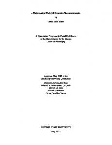
Figure 1: Time plots of model 2 with different initial conditions for 𝑅0 < 1. (a) Potential smokers; (b) smokers; (c) temporary quitters; (d) permanent quitters.
𝑔3 =
𝑓2 (𝑆, 𝑄𝑡 ) 𝑓1 (𝑃, 𝑄𝑡 ) − 𝑆𝑄𝑡 𝑃𝑄𝑡
=−
Using the normal vector 𝑛⃗ = (1, (𝜇 + 𝛾𝜎)/𝜇, 1) to Γ∗ , we can see that
(𝜇 + 𝛾) 𝛽 𝛽 (𝜇 + 𝛾𝜎) 𝑆 + −𝛽− 𝑄𝑡 𝑄𝑡 𝜇𝑄𝑡
(curl 𝑔) ⋅ 𝑛⃗ = −
𝜇 𝜇 𝛽𝜇 +𝛼− + + 𝑃𝑄𝑡 𝑄𝑡 𝑄𝑡 (𝜇 + 𝛾𝜎) −
𝛽𝛾𝜎 𝛾 (1 − 𝜎) − 𝜇𝑄𝑡 𝑃𝑄𝑡2
𝜇 + 𝛾𝜎 𝜇 𝛼𝛾𝜎 − 2 − 2 − < 0. 𝑃 𝑄𝑡 𝑃𝑆 𝜇𝑃
𝛽𝜇𝑃 𝛽𝜇 − . 𝑄𝑡 (𝜇 + 𝛾𝜎) (𝜇 + 𝛾𝜎)
(23)
Hence, model 3 has no periodic solutions, homoclinic loops, and oriented phase polygons inside the invariant region Γ∗ . (21)
Since the alternate forms of 𝑓1 , 𝑓2 , and 𝑓3 are equivalent in Γ, then 𝑔 ⋅ 𝑓 = 𝑔1 𝑓1 + 𝑔2 𝑓2 + 𝑔3 𝑓3 =
𝑓3 𝑓1 𝑓2 𝑓1 𝑓1 𝑓2 𝑓3 𝑓2 − + − 𝑃𝑄𝑡 𝑃𝑆 𝑃𝑆 𝑆𝑄𝑡 𝑓𝑓 𝑓𝑓 + 2 3 − 1 3 = 0. 𝑆𝑄𝑡 𝑃𝑄𝑡
So 𝑔 ⋅ 𝑓 = 0 on Γ∗ .
(22)
Consequently, we have the following result. Theorem 9 (global stability of 𝐸∗ ). If 𝑅0 > 1, then the smoking-present equilibrium point 𝐸∗ of system (3) is globally asymptotically stable. Proof. We know that, if 𝑅0 > 1 in Γ∗ , then 𝐸0 is unstable. Also Γ∗ is a positively invariant subset of Γ and the 𝜔 limit set of each solution of (3) is a single point in Γ∗ since there is no periodic solutions, homoclinic loops, and oriented phase
6
ISRN Applied Mathematics
0.25
0.7
Smokers S(t)
Potential smokers P(t)
0.8
0.6 0.5
0.20 0.15 0.10
0.4
0.05 0
20
40
60 80 100 Time (month)
120
140
0
20
40
60 80 100 Time (month)
(a)
120
140
(b)
Permanent quitters Qp (t)
Temporary quitters Qt (t)
0.25 0.25 0.20 0.15 0.10 0.05 0
20
40
60 80 100 Time (month)
120
140
3 4
1 2 (c)
0.20 0.15 0.10 0.05
20
0
40
60 80 100 Time (month)
120
140
3 4
1 2 (d)
Figure 2: Time plots of model 2 with different initial conditions for 𝛽 ⩾ 𝛼. (a) Potential smokers; (b) smokers; (c) temporary quitters; (d) permanent quitters.
polygons inside Γ∗ . Therefore 𝐸∗ is globally asymptotically stable.
5. Numerical Simulations In this section, we illustrate some numerical solutions of model 2 for different values of the parameters, and we show that these solutions are in agreement with the qualitative behavior of the solutions. We use the following parameters: 𝜇 = 0.04, 𝛾 = 0.3, 𝛼 = 0.25, and 𝜎 = 0.4, with two different values of the contact rate between potential smokers and smokers: for 𝑅0 < 1 we use 𝛽 = 0.2 and for 𝛽 ⩾ 𝛼 we use 𝛽 = 0.5. Model 2 is simulated for the following different initial values such that 𝑃 + 𝑆 + 𝑄𝑡 + 𝑄𝑝 = 1: (1) 𝑃(0) = 0.80301, 𝑆(0) = 0.10628, 𝑄𝑡 (0) = 0.08260, and 𝑄𝑝 (0) = 0.00811; (2) 𝑃(0) = 0.75000, 𝑆(0) = 0.16772, 𝑄𝑡 (0) = 0.07000, and 𝑄𝑝 (0) = 0.01228; (3) 𝑃(0) = 0.70000, 𝑆(0) = 0.21800, 𝑄𝑡 (0) = 0.05566, and 𝑄𝑝 (0) = 0.02634;
(4) 𝑃(0) = 0.63400, 𝑆(0) = 0.28800, 𝑄𝑡 (0) = 0.04800, and 𝑄𝑝 (0) = 0.03000. For 𝑅0 = 0.588235 < 1, Figure 1(a) shows that the number of potential smokers increases and approaches the total population 1. Figure 1(b) shows that the number of the smokers decreases and approaches zero. In Figures 1(c) and 1(d), temporary quitters and permanent quitters increase at first; after that they decrease and approach zero. We see from Figure 1 that, for any initial value, the solution curves tend to the equilibrium 𝐸0 , when 𝑅0 < 1. Hence, model 2 is locally asymptotically stable about 𝐸0 for the previous set of parameters. In Figure 2, we use the same parameters and initial values as previously with 𝛽 = 0.5. Figure 2(a) shows that the number of potential smokers decreases at first; then it increases and approaches 𝑃∗ . Figure 2(b) shows that the number of smokers increases at first; then it decreases and approaches 𝑆∗ . In Figures 2(c) and 2(d), temporary quitters and permanent quitters increase at first; after that they decrease and approach 𝑄𝑡∗ and 𝑄𝑝∗ . We see from Figure 2 that, for any initial value, the solution curves tend to the equilibrium 𝐸∗ , when 𝛽 ⩾ 𝛼.
ISRN Applied Mathematics Hence, model 2 is locally asymptotically stable about 𝐸∗ for the above set of parameters.
6. Discussion and Conclusions In this paper, we presented a mathematical model to analyze the behavior of smoking dynamics in a population with peer pressure effect on temporary quitters 𝑄𝑡 . Local asymptotic stability for the smoking-free equilibrium state is obtained when the threshold quantity 𝑅0 is less than 1 (i.e., when the contact rate 𝛽 between potential smokers and smokers is less than the sum of natural death rate 𝜇 and the quitting rate 𝛾). A Lyapunov function is used to show global stability of the smoking-free equilibrium when the contact rate between potential smokers and smokers is less than or equal to the natural death rate (𝛽 ≤ 𝜇). This means that the number of smokers may be controlled by reducing the contact rate 𝛽 to be less than the natural death rate 𝜇. On the other hand, if 𝛽 ⩾ 𝛼 (i.e., when the contact rate 𝛽 between potential smokers and smokers is greater than the contact rate 𝛼 between smokers and temporary quitters who revert back to smoking), then the smoking-present equilibrium state is locally asymptotically stable. By showing that this model has no periodic solutions, homoclinic loops, and oriented phase polygons inside the invariant region Γ∗ , we proved the global asymptotic stability of 𝐸∗ . This means that, if 𝑅0 > 1, smoking will persist. Some numerical simulations are performed to illustrate the findings of the analytical results. For 𝑅0 > 1, the results show that the smokers population reaches a steady state of approximately 6% of the total population. This model may be extended to include, for example, smokers who after quitting smoking may become potential smokers again. We may also consider the public health impact of smoking related illnesses as well.
Conflict of Interests The authors declare that there is no conflict of interests regarding the publication of this paper.
References [1] M. M. Bassiony, “Smoking in Saudi Arabia,” Saudi Medical Journal, vol. 30, no. 7, pp. 876–881, 2009. [2] “World Health Organization report on tobacco,” 2012, http://www.who.int/mediacentre/factsheets/fs339/en/. [3] C. Castillo-Garsow, G. Jordan-Salivia, and A. R. Herrera, “Mathematical models for the dynamics of tobacco use, recovery, and relapse,” Technical Report Series BU-1505-M, Cornell University, Ithaca, NY, USA, 1997. [4] O. Sharomi and A. B. Gumel, “Curtailing smoking dynamics: a mathematical modeling approach,” Applied Mathematics and Computation, vol. 195, no. 2, pp. 475–499, 2008. [5] A. Lahrouz, L. Omari, D. Kiouach, and A. Belmaˆati, “Deterministic and stochastic stability of a mathematical model of smoking,” Statistics & Probability Letters, vol. 81, no. 8, pp. 1276– 1284, 2011.
7 [6] G. Zaman, “Qualitative behavior of giving up smoking models,” Bulletin of the Malaysian Mathematical Sciences Society, vol. 34, no. 2, pp. 403–415, 2011. [7] G. Zaman, “Optimal campaign in the smoking dynamics,” Computational and Mathematical Methods in Medicine, vol. 2011, Article ID 163834, 9 pages, 2011. [8] V. S. Ert¨urk, G. Zaman, and S. Momani, “A numeric-analytic method for approximating a giving up smoking model containing fractional derivatives,” Computers & Mathematics with Applications, vol. 64, no. 10, pp. 3065–3074, 2012. [9] P. van den Driessche and J. Watmough, “Reproduction numbers and sub-threshold endemic equilibria for compartmental models of disease transmission,” Mathematical Biosciences, vol. 180, pp. 29–48, 2002. [10] F. Brauer, P. van den Driessche, and J. Wu, Mathematical Epidemiology, vol. 1945 of Lecture Notes in Mathematics, Springer, Berlin, Germany, 2008. [11] L. Perko, Differential Equations and Dynamical Systems, vol. 7 of Texts in Applied Mathematics, Springer, New York, NY, USA, 1991. [12] L. Cai, X. Li, M. Ghosh, and B. Guo, “Stability analysis of an HIV/AIDS epidemic model with treatment,” Journal of Computational and Applied Mathematics, vol. 229, no. 1, pp. 313– 323, 2009. [13] C. C. McCluskey and P. van den Driessche, “Global analysis of two tuberculosis models,” Journal of Dynamics and Differential Equations, vol. 16, no. 1, pp. 139–166, 2004. [14] J. Arino, C. C. McCluskey, and P. van den Driessche, “Global results for an epidemic model with vaccination that exhibits backward bifurcation,” SIAM Journal on Applied Mathematics, vol. 64, no. 1, pp. 260–276, 2003. [15] X. Ge and M. Arcak, “A sufficient condition for additive 𝐷stability and application to reaction-diffusion models,” Systems & Control Letters, vol. 58, no. 10-11, pp. 736–741, 2009. [16] M. W. Hirsch, S. Smale, and R. L. Devaney, Differential Equations, Dynamical Systems, and an Introduction to Chaos, vol. 60 of Pure and Applied Mathematics, Elsevier/Academic Press, Amsterdam, The Netherlands, 2nd edition, 2004. [17] S. Busenberg and P. van den Driessche, “Analysis of a disease transmission model in a population with varying size,” Journal of Mathematical Biology, vol. 28, no. 3, pp. 257–270, 1990.
Advances in
Hindawi Publishing Corporation http://www.hindawi.com
Algebra
Advances in
Operations Research
Decision Sciences
Volume 2014
Hindawi Publishing Corporation http://www.hindawi.com
Journal of
Probability and Statistics
Mathematical Problems in Engineering Volume 2014
Hindawi Publishing Corporation http://www.hindawi.com
Volume 2014
Hindawi Publishing Corporation http://www.hindawi.com
Volume 2014
The Scientific World Journal Hindawi Publishing Corporation http://www.hindawi.com
Hindawi Publishing Corporation http://www.hindawi.com
Volume 2014
International Journal of
Differential Equations Hindawi Publishing Corporation http://www.hindawi.com
Volume 2014
Volume 2014
Submit your manuscripts at http://www.hindawi.com International Journal of
Advances in
Combinatorics
Mathematical Physics
Volume 2014
Hindawi Publishing Corporation http://www.hindawi.com
Journal of
Complex Analysis Hindawi Publishing Corporation http://www.hindawi.com
Volume 2014
International Journal of Mathematics and Mathematical Sciences
Hindawi Publishing Corporation http://www.hindawi.com
Journal of
Hindawi Publishing Corporation http://www.hindawi.com
Stochastic Analysis
Abstract and Applied Analysis
Hindawi Publishing Corporation http://www.hindawi.com
Hindawi Publishing Corporation http://www.hindawi.com
International Journal of
Mathematics Volume 2014
Volume 2014
Journal of
Volume 2014
Discrete Dynamics in Nature and Society Volume 2014
Hindawi Publishing Corporation http://www.hindawi.com
Journal of Applied Mathematics
Optimization
Hindawi Publishing Corporation http://www.hindawi.com
Hindawi Publishing Corporation http://www.hindawi.com
Volume 2014
Journal of
Discrete Mathematics
Journal of Function Spaces Hindawi Publishing Corporation http://www.hindawi.com
Volume 2014
Hindawi Publishing Corporation http://www.hindawi.com
Volume 2014
Hindawi Publishing Corporation http://www.hindawi.com
Volume 2014
Volume 2014
Volume 2014