Global Illumination with Radiance Regression Functions Peiran Ren∗‡ Jiaping Wang† ∗ Tsinghua University
Minmin Gong‡ Stephen Lin‡ † Microsoft Corporation
(a)
Xin Tong‡ Baining Guo‡∗ Research Asia
‡ Microsoft
(b)
(c)
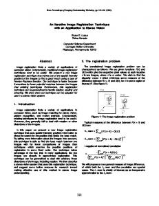
Figure 1: Real-time rendering results with radiance regression functions for scenes with glossy interreflections (a), multiple local lights (b), and complex geometry and materials (c).
Abstract We present radiance regression functions for fast rendering of global illumination in scenes with dynamic local light sources. A radiance regression function (RRF) represents a non-linear mapping from local and contextual attributes of surface points, such as position, viewing direction, and lighting condition, to their indirect illumination values. The RRF is obtained from precomputed shading samples through regression analysis, which determines a function that best fits the shading data. For a given scene, the shading samples are precomputed by an offline renderer. The key idea behind our approach is to exploit the nonlinear coherence of the indirect illumination data to make the RRF both compact and fast to evaluate. We model the RRF as a multilayer acyclic feed-forward neural network, which provides a close functional approximation of the indirect illumination and can be efficiently evaluated at run time. To effectively model scenes with spatially variant material properties, we utilize an augmented set of attributes as input to the neural network RRF to reduce the amount of inference that the network needs to perform. To handle scenes with greater geometric complexity, we partition the input space of the RRF model and represent the subspaces with separate, smaller RRFs that can be evaluated more rapidly. As a result, the RRF model scales well to increasingly complex scene geometry and material variation. Because of its compactness and ease of evaluation, the RRF model enables real-time rendering with full global illumination effects, including changing caustics and multiple-bounce high-frequency glossy interreflections. CR Categories: I.3.7 [Computer Graphics]: Three-Dimensional Graphics and Realism—Color, shading, shadowing, and texture; Links: DL PDF W EB
ACM Reference Format Ren, P., Wang, J., Gong, M., Lin, S., Tong, X., Guo, B. 2013. Global Illumination with Radiance Regression Functions. ACM Trans. Graph. 32, 4, Article 130 (July 2013), 12 pages. DOI = 10.1145/2461912.2462009 http://doi.acm.org/10.1145/2461912.2462009. Copyright Notice Permission to make digital or hard copies of all or part of this work for personal or classroom use is granted without fee provided that copies are not made or distributed for profit or commercial advantage and that copies bear this notice and the full citation on the first page. Copyrights for components of this work owned by others than ACM must be honored. Abstracting with credit is permitted. To copy otherwise, or republish, to post on servers or to redistribute to lists, requires prior specific permission and/or a fee. Request permissions from
[email protected]. Copyright © ACM 0730-0301/13/07-ART130 $15.00. DOI: http://doi.acm.org/10.1145/2461912.2462009
Keywords: global illumination, real time rendering, neural network, non-linear regression
1
Introduction
Global light transport provides scenes with visually rich shading effects that are an essential component of photorealistic rendering. Much of the shading detail arises from multiple bounces of light. This reflected light, known as indirect illumination, is generally expensive to compute. The most successful existing approach for indirect illumination is precomputed radiance transfer (PRT) [Sloan et al. 2002; Ramamoorthi 2009], which precomputes the global light transport and stores the resulting PRT data for fast rendering at run time. However, even with PRT, real-time rendering with dynamic viewpoint and lighting remains difficult. Two major challenges in real-time rendering of indirect illumination are dealing with dynamic local light sources and handling highfrequency glossy interreflections. Most existing PRT methods assume that the lighting environment is sampled at a single point in the center of the scene and the result is stored as an environment map. For this reason, these methods cannot accurately represent incident radiance of local lights at different parts of the scene. To address this problem, Kristensen et al. [2005] precomputed radiance transfer for a dense set of local light positions and a sparse set of mesh vertices. Their approach works well for diffuse scenes but has difficulty representing effects such as caustics and high-frequency glossy interreflections, since it would be prohibitively expensive to store the precomputed data for a dense set of mesh vertices. To face these challenges, we introduce the radiance regression function (RRF), a function that returns the indirect illumination value for each surface point given the viewing direction and lighting condition. The key idea of our approach is to design the RRF as a nonlinear function of surface point properties such that it has a compact representation and is fast to evaluate. The RRF is learned for a given scene using nonlinear regression [Hertzmann 2003] on training samples precomputed by offline rendering. These samples consist of a set of surface points rendered with random viewing and lighting conditions. Since the indirect illumination of a surface point in a given scene is determined by its position, the location of light sources, and the viewing direction, we define these properties as basic attributes of the point and learn the RRF with respect to them. In rendering, the attributes of each visible surface point are obtained while evaluating direct illumination. The indirect illumiACM Transactions on Graphics, Vol. 32, No. 4, Article 130, Publication Date: July 2013
130:2
•
P. Ren et al.
nation of each point is then computed from their attributes using the RRF, and added to the direct illumination to generate a global illumination solution.
RRF representation is run-time local, i.e., the run-time evaluation of the RRFs of each 3D object is independent of the RRFs of other 3D objects in the scene.
We model the RRF by a multilayer acyclic feed-forward neural network. As a universal function approximator [Hornik et al. 1989], such a neural network can approximate the indirect illumination function to arbitrary accuracy when given adequate training samples. The main technical issue in designing our neural network RRF is how to achieve a good approximation through efficient use of the precomputed training samples. To address this issue we present two techniques. The first is to augment the set of attributes at each point to include spatially variant surface properties. Though regression could be performed using only the basic attributes, this results in suboptimal use of the training data and inferior approximation results because spatially variant surface properties make the RRF highly complex as a function of only the basic attributes. By performing regression with respect to an enlarged set of attributes that includes surface normal and material properties, the efficiency of sample use is greatly elevated because the mapping from the augmented attributes to indirect illumination can be much more easily computed from training samples. The second technique is to partition the space of RRF input vectors and fit a separate RRF for each of the subspaces. Though a single neural network can effectively model the indirect illumination of a simple scene, the larger network size needed to model complex scenes leads to substantially increased training and evaluation time. To expedite run-time evaluation, we employ multiple smaller networks that collectively and more efficiently represent indirect illumination throughout the scene.
2
Our main contribution is a fundamentally new approach for realtime rendering of precomputed global illumination. Our method directly approximates the indirect global illumination, which is a highly complex and nonlinear 6D function (of surface position, viewing direction, and lighting direction). With carefully designed neural networks, our method can effectively exploit the nonlinear coherence of this function in all six dimensions simultaneously. By contrast, PRT methods only exploit nonlinear coherence in some dimensions and resort to dense sampling in the other dimensions. Run-time evaluation of analytic neural-network RRFs can be accomplished in screen space with a deferred shading pass easily integrated into existing rendering pipelines. As a result, the precomputed RRFs are both compact and fast to evaluate, and our method can render challenging visual effects - such as caustics, sharp indirect shadows, and high-frequency glossy interreflections - all in real time. In our method the precomputed neural networks depend only on lighting effects on the object surface, not on the underlying surface meshing. This makes our method more scalable than PRT, which relies on dense surface meshing for high-frequency lighting effects. As far as we know, our method provides the first real-time solution for rendering full indirect illumination effects of complex scenes with dynamic local lighting and viewing. For scenes with complex geometry and material variations (e.g., Figure 1), our technique can render their full global illumination effects in 512 × 512 images at 30 FPS, capturing visual effects such as caustics (Figure 9(a)), high-frequency glossy interreflections (Figure 8(d)), glossy interreflections produced by four or more light bounces (Figure 1(a) and Figure 10), indirect hard shadows (Figure 1(c)), and mixtures of different lighting effects in complex scenes (Figure 12). The rendering time mainly depends on the screen size, not the number of objects in the scene. It is fairly easy to scale up to larger scenes with many objects because our run-time algorithm renders all visible objects in parallel in screen space. This scalability is reflected in our results, where the frame rates of the complex bedroom scene (Figure 12) and the simple Cornell box (Figure 9(a)) are about the same. Our ACM Transactions on Graphics, Vol. 32, No. 4, Article 130, Publication Date: July 2013
Related Work
Due to space limitations, we only discuss recent methods that are directly related to our work. For a broader presentation on interactive global illumination techniques, we refer the reader to recent surveys [Wald et al. 2009; Ramamoorthi 2009; Ritschel et al. 2012]. Numerous methods have been proposed to quickly compute the global illumination of a scene. One solution is to accelerate classical global illumination algorithms using the GPU or multiple CPUs [Wald et al. 2009]. Recently, Wang et al. [2009] presented a GPU based photon mapping method for rendering full global illumination effects. McGuire et al. [2009] developed an image space photon mapping algorithm to exploit both the CPU and GPU for global illumination. Parker et al. [2010] described a programmable ray tracing engine designed for the GPU and other highly parallel architectures. Interactive Global Illumination
Another approach for obtaining real-time frame rates is to sacrifice accuracy for speed. One such solution is to approximate indirect lighting reflected from surfaces as a set of virtual point lights (VPLs) [Keller 1997; Dachsbacher and Stamminger 2006; Ritschel et al. 2008; Nichols and Wyman 2010; Thiedemann et al. 2011]. Several methods [Dong et al. 2007; Dachsbacher et al. 2007; Crassin et al. 2011] approximate global illumination using coarsescale solutions computed over a scene hierarchy. More recently, Kaplanyan et al. [2010] approximated low frequency indirect illumination in dynamic scenes by computing light propagation over a 3D scene lattice. While this method is fast and compact, it can only simulate indirect illumination of diffuse surfaces. Despite the different strategies used for speeding up computation, the processing costs of these methods remain proportional to the number of light bounces, which effectively limits the interreflection effects they can simulate. As the scene geometry becomes more complex and the material becomes more glossy, the diverse light paths often lead to greater computational costs in each bounce, which also limits the scalability of these methods. On the contrary, our method efficiently models all indirect lighting effects, including challenging effects such as caustics and high-frequency glossy interreflections. Precomputed radiance transfer (PRT) [Sloan et al. 2002; Ng et al. 2004; Ramamoorthi 2009] precomputes the light transport of each scene point with respect to a set of basis illuminations, and uses this data at run time to relight the scene at real-time rates. Early methods [Sloan et al. 2002; Sloan et al. 2003] support only low-frequency global illumination effects by encoding the light transport with a spherical harmonics (SH) basis. Later methods factorize the BRDF at each surface point and represent the light transport with non-linear wavelets [Liu et al. 2004; Wang et al. 2006] or a spherical Gaussian basis [Tsai and Shih 2006; Green et al. 2006] for rendering all-frequency global illumination. However, these methods are limited by their support for only distant lighting. Precomputed Light Transport
To support local light sources, Kristensen et al. [2005] model reflected radiance using a 2D SH basis, with sampling at a sparse set of mesh vertices for a dense set of local light positions. The light space samples are compressed by clustering, while the spatial samples are partitioned into zones and compressed using clustered PCA. During rendering, the data sampled at nearby light sources are interpolated to generate rendering results for a new light position.
Global Illumination with Radiance Regression Functions
Since the data is sampled over sparse mesh vertices, this method cannot well represent caustics and other high-frequency lighting effects. Also, a high-order SH basis is needed for representing viewdependent indirect lighting effects on glossy objects. Direct-to-indirect transfer methods [Haˇsan et al. 2006; Wang et al. 2007; Kontkanen et al. 2006; Lehtinen et al. 2008] precompute indirect lighting with respect to the direct lighting of the scene at sampled surface locations. During rendering, the direct shading of the scene is first computed and then used to reconstruct the indirect lighting effects. Although this method can support local light sources, the surfaces must be densely sampled to represent highfrequency indirect lighting, which leads to large storage costs and slow rendering performance. Regression methods have been widely used in graphics [Hertzmann 2003]. For example, Grzeszczuk et al. [1998] used neural networks to emulate object dynamics and generate physically realistic animation without simulation. Neural networks also have been used for visibility computation. Dachsbacher [2011] applied neural networks for classifying different visibility configurations. Nowrouzezahrai et al. [2009] fit lowfrequency precomputed visibility data of dynamic objects with neural networks. These visibility neural networks allow them to predict low-frequency self-shadowing when computing the direct shading of a dynamic scene. Finally, Meyer et al. [2007] used statistical methods to select a set of key points (hundreds of them) and form a linear subspace such that at run time, global illumination only needs to be calculated at these key points. Although this method greatly reduces computation, rendering global illumination at key points remains time consuming.
Regression Methods
3
Radiance Regression Functions
In this section, we first present the radiance regression function Φ and explain how it can be obtained through regression with respect to precomputed indirect illumination data. Then we describe how to model the function Φ as a neural network ΦN and derive an analytic expression for the function ΦN . After that, we discuss neural network structure and training, leaving the more technical details to Appendix A. Finally, we show a simple example of rendering with the function ΦN . In a static scene lit by a moving point light source, the reflected radiance at an opaque surface point at position x p as viewed from direction v is described by the reflectance equation [Cohen et al. 1993]: Z
s(x p , v, l) =
Ω+ 0
ρ(x p , v, vi )(n · vi )si (x p , vi )dvi
(1)
=s (x p , v, l) + s+ (x p , v, l), where l is the position of the point light, ρ and n denote the BRDF and surface normal at position x p , and si (x p , vi ) represents the incoming radiance at x p from direction vi . The parametric BRDF ρ can be described by a closed-form function ρc with a set of reflectance parameters a(x p ) as follows: ρ(x p , v, vi ) = ρc (v, vi , a(x p )).
(2)
For a spatially variant parametric BRDF, the only part that varies spatially is the parameter vector a(x p ), which is represented by a set of texture maps and thus can be efficiently used in the graphics pipeline. As shown in Equation (1), the reflected radiance s can be separated into a local illumination component s0 and indirect illumination component s+ that correspond to direct and indirect lighting
•
130:3
respectively. As the local illumination component s0 can be efficiently computed by existing methods (e.g. [Donikian et al. 2006]), we focus on the indirect illumination s+ that results from incoming radiance contributions to si (x p , vi ) of indirect lighting. Given a point light of unit intensity at position l, the function s+ (x p , v, l) represents the indirect illumination component toward viewing direction v. Combining Equation (1) and Equation (2), we can express the indirect illumination component as s+ (x p , v, l) =
Z Ω+
ρc (v, vi , a(x p ))(n(x p ) · vi )s+ i (x p , vi )dvi
(3)
where s+ i (x p , vi ) is the indirect component of the incoming radiance si (x p , vi ). Here we also replaced the surface normal n by n(x p ) to make explicit the fact that the surface normal n at position x p is computed as a function of x p . From Equation (3) we observe that the indirect illumination s+ may be rewritten as s+ (x p , v, l) = s+ a (x p , v, l, n(x p ), a(x p )),
(4)
for a new function s+ a with an expanded set of attributes that includes the surface normal and BRDF parameter vector. The indirect illumination s+ (x p , v, l) is a well-defined function since for a given scene, we can perform light transport computation to obtain s+ for any surface point, light position, and viewing direction. However, s+ generally requires lengthy processing to compute. In this work, we introduce the radiance regression function Φ, which is a function that approximates s+ in the least-squares sense and is constructed such that it is compact, fast to evaluate, and hence well-suited for real-time rendering. Approximation by Regression We treat the approximation of indirect illumination s+ as a regression problem [Hertzmann 2003] and learn a regression function Φ from a set of training data. In principle, it would be sufficient to define Φ in terms of only the set of basic attributes x p , v and l, since they describe a minimal set of factors that determine the indirect illumination at a point in a given scene. However, the values of surface normals n and reflectance parameters a can vary substantially over a scene area, making indirect illumination s+ (x p , v, l) highly complex as a function of only the basic attributes. Defining the regression function Φ in terms of a set of augmented attributes x p , v, l, n, and a thus allows for more effective approximation of s+ by nonlinear regression, since the surface quantities n and a would no longer need to be inferred from the training data. We therefore define the radiance regression function Φ at surface point p to be Φ(x p , v, l, n, a), which represents a map from R12+n p to R3 where n p is the number of parameters in the spatially variant BRDF and R3 spans the three RGB color channels. The training data we use consists of a set of N input-output pairs that sample the indirect illumination s+ (x p , v, l). Each pair is called an example, and the i-th example comprises the pair (xi , yi ), where xi = [xip , vi , li , ni , ai ]T , yi = s+ (xip , vi , li ), and i = 1, ..., N. xi is the input vector and yi is the corresponding output vector. The radiance regression function Φ is determined by minimizing the leastsquares error: E = ∑ ||yi − Φ(xip , vi , li , ni , ai )||2 .
(5)
i
There may exist many functions that pass through the training points (xi , yi ) and thus minimize Equation (5). A particular solution might give a poor approximation of the indirect illumination s+ (x p , v, l) at a new input vector (x p , v, l, n, a) unseen in the training data. To produce a better approximation, a larger training set ACM Transactions on Graphics, Vol. 32, No. 4, Article 130, Publication Date: July 2013
130:4
•
P. Ren et al.
Each node operates by taking inputs from the preceding layer and computing an output based on components {wijk } of the weight vector w. Let us consider node j in the i-th layer, with nij denoting its output and wij0 as its bias weight. For each hidden layer, nij is calculated from the outputs of all nodes in the (i − 1)-th layer as follows: nij = σ (zij ), zij = wij0 +
∑ wijk ni−1 k ,
(7)
k>0
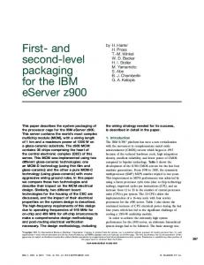
Figure 2: Modeling the RRF by an acyclic feed-forward neural network, which defines a mapping from the input vector (x p , v, l, n, a) to the output RGB components defined in Equation (8).
size N could be used to more densely sample the input space. However, N must be limited in practice and to obtain a useful regression function Φ we must restrict the eligible solutions for Equation (5) to a smaller set of functions. These restricted models are known as structured regression models [Hastie et al. 2009]. One of the simplest is the linear model, which would work poorly for indirect illumination s+ (x p , v, l) as it is highly non-linear with respect to its input vector (x p , v, l, n, a). In this work, we choose a neural network as our regression model. The primary reason for choosing neural networks is their relative compactness and high speed in evaluation, which are critical factors for real-time rendering. Neural networks also are well-suited for our problem because they provide a simple yet powerful non-linear model that has been shown to compete well with the best methods on regression problems. A neural network may be regarded as a non-linear generalization of the linear regression model as we shall see. Moreover, neural networks have strong representational power and have been widely used as universal function approximators. Specifically, continuous functions or square-integrable functions on finite domains can be approximated with arbitrarily small error by a feed-forward network with one or two hidden layers [Hornik et al. 1989; Blum and Li 1991]. The indirect illumination function s+ belongs to this category of functions. Neural Network RRF With the radiance regression function represented by a neural network, we rewrite the RRF as ΦN (x p , v, l, n, a, w), where the new vector w is the weight vector of the neural network ΦN and the components of w are called weights of ΦN . Now Equation (5) becomes E(w) = ∑ ||yi − ΦN (xip , vi , li , ni , ai , w)||2 .
(6)
i
To find ΦN , we need to select the structure of the neural network and then determine its weights by minimizing E(w). A neural network is a weighted and directed graph whose nodes are organized into layers. The weights of the edges constitute the components of the weight vector w. The network we use is an acyclic feed-forward network with two hidden layers, as shown in Figure 2. Each node is connected to all nodes of the preceding layer by directed edges, such that a node in the i-th layer receives inputs from all nodes in the (i − 1)-th layer. The graph takes inputs through the nodes in the first layer, also known as the input layer, and produces outputs through the nodes in the last layer, the output layer. The nodes in the input layer correspond to the dimensions of the RRF’s input vector (x p , v, l, n, a). The output layer consists of three nodes, one for each of the RGB color channels of the indirect illumination s+ . The layers between the input and output layers are called the hidden layers. ACM Transactions on Graphics, Vol. 32, No. 4, Article 130, Publication Date: July 2013
where wijk is the weight of the directed edge from node k of the preceding layer to node j in the current layer. The node outputs the value σ (zij ) where σ is the hyperbolic tangent function σ (z) = tanh(z) = 2/(1 + e−2z ) − 1, and zij is a linear combination of outputs from the preceding layer. The hyperbolic tangent function is equivalent to the equally popular sigmoid function σ1 (z) = 1/(1 + e−z ). Both σ and σ1 resemble the step function (the Heaviside function) except that σ and σ1 are continuous and differentiable, which greatly facilitates numerical computation. For the output layer, nij is simply nij = wij0 + ∑k>0 wijk ni−1 k . Let ΦN = [Φ1N , Φ2N , Φ3N ] and x = [x p , v, l, n, a]. From Equation (7), we obtain the analytic expression for ΦN as follows: 9
ΦiN (x, w) = w3i0 + ∑ w3i j σ (w2j0 + ∑ w2jk σ (w1k0 + ∑ w1kl xl )), (8) j>0
k>0
l=1
where i = 1, 2, 3 and xl is the l-th component of the input vector x. Note that the hyperbolic tangent function σ is the only nonlinear element of ΦN . Indeed, if we replace all hyperbolic tangent functions in ΦN by linear functions, then ΦN becomes a linear model. In this sense, a neural network is a nonlinear generalization of the simple linear regression model. Neural Network Structure & Training We choose the neural network structure shown in Figure 2 based on the following considerations. Since the input and output layers are fixed according to the input and output format, only the number of hidden layers and the number of nodes in each hidden layer need to be determined. In theory, a neural network with one hidden layer can approximate a continuous function to arbitrary accuracy [Hornik et al. 1989]. However, the indirect illumination function s+ contains many ridges and valleys. This type of function requires a large number of nodes to approximate if only one hidden layer is used, whereas with two hidden layers such functions can be effectively approximated by a relatively small number of nodes [Chester 1990; FAQ ]. Note that discontinuities in the indirect illumination s+ are not a problem because with large weights the hyperbolic tangent function essentially becomes a step function. Neural networks with more than two hidden layers are typically not used for function approximation because they are difficult to train. In Appendix A, we discuss how we set the number of nodes in the two hidden layers. The neural network ΦN is trained by using numerical optimization to find the weights in w that minimize E(w) as defined in Equation (6) for the training set. This training set is constructed by sampling light positions and viewpoints, and tracing rays from the viewpoint towards points in the scene to determine their indirect illumination. The number of training samples is roughly ten times the number of weights in w. Details on the training process and issues such as overfitting are described in Appendix A. Rendering After training the neural network, the indirect illumination of each scene point can be rendered under different lighting and viewing conditions. For a given viewpoint and light position, we first compute the visible surface points of each screen pixel and their surface position x p . Each attribute in the input vector is scaled to [−1.0, 1.0]. Then for each pixel, the scaled input vector
Global Illumination with Radiance Regression Functions
(a)
•
130:5
(b)
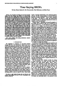
Figure 4: Partitioning of input space for fitting of multiple RRFs.
4
(c)
(d)
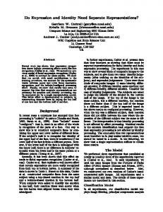
Figure 3: Comparison of RRFs with/without surface normal and SVBRDF attributes. (a) Ground truth by path tracing. (b) RRFs with augmented attributes, including both surface normal and SVBRDF parameters. (c) RRFs with basic attributes plus only SVBRDF parameters. (d) RRFs with only basic attributes (no surface normal or SVBRDF parameters).
(x p , v, l, n, a) is input to the neural network ΦN to compute the indirect illumination value. These indirect illumination results are then added to those of direct illumination to generate the final rendering. Run-time evaluation of ΦN is easy because both a(x p ) and n(x p ) can be made available in the graphics pipeline. As mentioned earlier, a(x p ) is stored as a set of texture maps and is thus accessible through texture mapping. n(x p ) is also available because it is calculated in evaluating the direct illumination s0 in Equation (1). By contrast, other factors that affect indirect illumination, such as the distance and angles of other scene points, are relatively unsuitable for inclusion in the input vector. Not only are these quantities not readily available in the graphics pipeline, but they would require a substantial number of inputs to represent, which would significantly increase the number of neural network weights that need to be learned. Each additional input adds n1 weights to the neural network, where n1 is the number of nodes in the first hidden layer. Since our design principle for the RRF is to make it compact and fast to evaluate, we limit the number of additional inputs and only choose quantities that are readily available. Figure 3 displays rendering results of a simple scene consisting of two objects, a sphere and a box, each of which is modeled by an RRF. The ground truth image in (a) was rendered with the physically-based offline path tracer [Lafortune and Willems 1993] used in generating the training data. Here the sphere is textured by a normal map and a spatially variant isotropic Ward BRDF [Ward 1992], whose spatially variant parameter a(x p ) is a 7D vector consisting of 3D diffuse and specular colors and 1D specular roughness. The same training data set is used to generate (b), (c) and (d). In comparison to RRFs with only basic attributes (d) or basic attributes plus only SVBRDF parameters (c), the inclusion of both surface properties among the augmented attributes leads to higher fidelity reproduction of surface details (b). Other frequently-used parametric BRDF models such as the Cook-Torrance model, BlinnPhong model, anisotropic Ward model, and Ashikhmin-Shirley model can also be effectively utilized in this manner.
Handling Scene Complexity
Input Space Partitioning So far, we have not considered complex scenes with many objects. In theory, such a scene could be approximated by a single RRF with a large number of nodes in the hidden layers. However, this significantly complicates RRF training, as the number of weights to be learned increases quadratically with the number of hidden-layer nodes. More importantly, a larger network leads to a much greater evaluation cost, which also increases quadratically with the number of hidden-layer nodes. As a result, expanding the neural network quickly becomes infeasible for realtime rendering. We address this issue by decomposing the space spanned by neural network input vectors into multiple regions and fitting a separate RRF to the training data of each region. To partition the input space, we take advantage of the fact that the scene is already divided into different 3D objects as part of the content creation process (typically each object is topologically disconnected from other objects in the scene). For each 3D object, we subdivide its input space using a kd-tree, which is a binary tree suitable for recursive subdivision of a high-dimensional space. With this partition, the computation of the indirect illumination value for an input only involves a kd-tree search, which is extremely fast, and an evaluation of a small RRF. For each object, its input space is an n-dimensional box, and we denote its kd-tree as Σ. Every non-leaf node ν in Σ is an n-dimensional point, which implicitly generates a splitting hyperplane that divides the current-level box into two boxes at the next level of the kd-tree. Each non-leaf node is associated with one of the n dimensions xi , such that the splitting hyperplane is perpendicular to that dimension’s axis. For simplicity we always split the current-level box through the middle, generating two next-level boxes of equal size. The box to the left of the splitting hyperplane belongs to the left subtree of node ν, and the box to the right belongs to the right subtree. Finally, the leaf nodes of the kd-tree Σ hold boxes that are not subdivided further. Figure 4 illustrates the subdivision processing at a node ν, highlighted in (a). We take the training samples within the ndimensional box ω associated with the node ν and fit an RRF to them. To reduce discontinuity across adjacent boxes, we include additional training samples from neighboring boxes by expanding the box ω by 10% along each dimension as shown in (b). We could further reduce discontinuities across the boundary of adjacent boxes by creating a small transition zone and linearly interpolating the adjacent RRFs. However, through experiments we found this to be unnecessary. Before training, we normalize the bounding box of the samples to a unit hypercube as shown in (c-d). We stop subdividing the node ν when both training and prediction errors are less than 5% (relative error). Here the prediction error is measured by evaluating the RRF against a test set removed from the pool of all training samples. In our experiments, we remove 30% of the ACM Transactions on Graphics, Vol. 32, No. 4, Article 130, Publication Date: July 2013
130:6
•
P. Ren et al.
training samples for testing. If further subdivision of the node ν is required, we need to choose an axis xi for splitting ν. The best splitting axis is the one that generates the smallest training and prediction errors on the child nodes of ν. A brute-force way to find this axis is to try every axis and carry out the RRF fitting and testing process on the resulting child nodes. Alternatively, we could randomly select a splitting axis, which results in roughly 10% higher RRF fitting and testing errors in our experiments.1 For the results reported in this paper, we use the brute-force method to identify the splitting axis. The use of augmented attributes instead of only basic attributes increases the apparent dimensionality of the input space, which could make the subdivision process less efficient by creating a larger number of insignificant cells. However, we note that though s+ a appears to be a higher dimensional function than s+ , the intrinsic dimen+ sionality of s+ a is no greater than s because both a and n are not independent variables but rather functions of x p , which is already an attribute in the input vector of s+ . The function s+ a is simply the original function s+ embedded in a higher dimensional space. Since our kd-tree subdivision criteria is completely driven by fitting and prediction errors, a cell will be created only when necessary (i.e., when the errors are too high) and this fact remains true no matter which space s+ is embedded. This error-driven subdivision criteria ensures that no unnecessary cells are created. A benefit of using kd-trees over a quadtree/octree-like partitioning structure is that node splits are not jointly performed over all dimensions, which may lead to an overabundance of nodes in the high-dimensional space and hence many more RRFs than needed. Lighting Complexity Our discussion so far focuses on the case of a single point light source. It is straightforward to handle the general case of any finite number of local lights of any colors. More importantly, this can be done without recomputing the RRF ΦN . Suppose there are K light sources with the k-th light located at position lk . Since ΦN is computed for a unit light source and light transport is linear with respect to light intensities, the indirect illumination s+ may be written as s+ (x p , v, l1 , ..., lK ) =
k=K
∑ ck ΦN (x p , v, lk , n, a, w),
(9)
k=1
where ck is the color of the k-th light. This equation implies that the light positions and colors are all variables that are free to change independently under user control. Since each term in the sum is evaluated by the same RRF ΦN , no additional training or storage cost is needed for multiple point lights. At run time, the main cost is the evaluation of ΦN for multiple light positions and the computation of direct illumination for each of the lights. Note that the linearity of light transport allows us to handle any finite number of local lights of any colors by using the same RRF ΦN . Without this property, we would have to simultaneously include the positions and colors of all lights as input variables of ΦN , resulting in a neural network that is prohibitively expensive to train and store.
5
Implementation and Results
We implemented the proposed partitioning and training algorithm on a PC cluster with 200 nodes, each of which is configured with 1 Note that these errors are only used for guiding the subdivision of nonleaf nodes; the final fitting and testing errors on the leaf nodes are determined by the same stopping criteria no matter how splitting axes are chosen.
ACM Transactions on Graphics, Vol. 32, No. 4, Article 130, Publication Date: July 2013
Scene CornellBox Plant Kitchen Sponza Bedroom
Vertex Num. 29K 194K 122K 31K 194K
Sample Num. 10M 110M 60M 50M 190M
Partition Num. 6.5K 75.5K 32.5K 33.0K 127.4K
Sampling Time 0.25h 3h 12h 2.5h 75h
Training Time 0.75h 7.5h 1.5h 1.2h 10h
Table 1: Performance data on RRF training. Scene CornellBox Plant Kitchen Sponza Bedroom
RRF Size 5.64MB 66.77MB 33.12MB 24.81MB 109.09MB
FPS 61.9fps 32.6fps 36.5fps 60.8fps 69.1fps
Dir. Shading 5.33ms 5.10ms 15.341ms 6.75ms 2.61ms
Tree Trav. 2.39ms 2.52ms 2.37ms 2.16ms 2.44ms
RRF Eval. 8.43ms 23.05ms 9.62ms 7.54ms 9.40ms
Table 2: Performance data on RRF-based rendering. Dir. shading denotes the computation time for direct shading. Tree Trav. is the computation time for partition tree traversal, and RRF Eval. represents the time for RRF evaluation. two Quadcore Intel Xeon L5420 2.50G CPUs and 16GB of memory. The indirect illumination values for the training set are computed using the Mitsuba renderer [Jakob 2010] on the same cluster. The real-time rendering algorithm is implemented on an nVidia GeForce GTX 680 with 2GB of video memory. The direct illumination component is calculated with a programmable rendering pipeline using variance shadow maps [Donnelly and Lauritzen 2006]. At run time, we use CUDA to compute the indirect illumination value for each screen pixel as follows. The input vectors of all pixels are stored in a matrix M that is converted from the G-buffers of the deferred shading pipeline, one input vector per matrix column. Since a kd-tree is built for each 3D object, we also store an object ID with each input vector so that it is easy to locate the corresponding kd-tree. In the CUDA kernel for kd-tree traversal, each thread reads an input vector x from the matrix M, locates a kd-tree, and traverses down the kd-tree to reach a leaf node, where it picks up the ID of the neural network ΦN for the partition containing x. Then in the neural network CUDA kernel, each thread feeds the input vector x to the neural network ΦN and evaluates the color value of the pixel according to Equation (8). We tested our method on a variety of scenes that exhibit different light transport effects. The Cornell Box scene (Figure 9 a-b) includes rich interreflection effects between the diffuse and specular surfaces, such as color bleeding and caustics. In the Plant scene (Figure 9 c-d), the fine geometry of the plant model results in complex occlusions and visibility change. The Kitchen scene (Figure 10) is used to illustrate view-dependent indirect illumination effects caused by strong interreflections between specular surfaces. We also tested the scalability of our method on two complex scenes. The Sponza scene (Figure 11) consists of diffuse surfaces with complex geometry. In the Bedroom scene (Figure 12), objects with different shapes and material properties are placed together and they present rich and complicated shading variations under different lighting and viewing conditions. Table 1 lists for each scene the number of vertices and detailed training performance data, including training data sizes and timings for training sample generation and the training process.The Scene CornellBox Plant Kitchen
Mean error 0.029 0.066 0.056
Random training set 0.00021 0.00014 0.00008
Random weight init. 0.00018 0.00014 0.00032
Table 3: Rendering accuracy of three scenes, and robustness with respect to different choices of training data set and different initial neural network weight values.
Global Illumination with Radiance Regression Functions
(a)
(b)
(e)
(c)2.5M
(e)40M
(f)Traced
130:7
(c) (d)10M
(d)
(a) (b)0.625M
•
(f)
Figure 6: Accuracy of RRFs generated from training sets of different sizes. (a) Rendering errors of RRFs computed from different sizes of training data. (b)-(e) Rendering results of the different RRFs. (f) Ground truth image. (g)
(h)
(i)
Figure 5: Comparison of results rendered by our method and those of path tracing. Only indirect illumination results are shown. Left: Path tracing results. Middle: Our rendering results. Right: Difference between the two results. run-time rendering performance for each scene is reported in Table 2. The relatively long RRF evaluation time for the Plant scene is due to its intricate geometry, which leads to many neighboring points belonging to different partitions and hence low data coherence. The image resolution for all the renderings is 512 × 512. We validate our RRF training and rendering method with the Cornell Box, Plant and Kitchen scenes. To evaluate accuracy, we compare the images rendered by our method to ground truth images generated by Mitsuba path tracing with each pixel rendered using 16384 rays for the Cornell Box scene, 4096 rays for the Plant scene, and 32768 rays for the Kitchen scene. In this experiment, we rendered 400 images of 512 × 512 resolution with pairings between 20 randomly selected view positions and 20 random light positions, none of which were used in the training set. The rendering error E was computed as the root-mean-square error of the 400 image pairs. The first column of Table 3 shows the mean errors for three scenes. Figure 5 shows our results, the ground truth images, and the differences between them. It is seen that the RRFs accurately predict the indirect illumination values of surface points under novel lighting, and they generate results that are visually similar to the ground truth. Note that the errors in textured regions are mainly due to the different texture filters used in Mitsuba and our RRF rendering, while the errors along object boundaries are caused by the single sample ray for each pixel used in our RRF rendering. Method Validation
To test the robustness of our training method with different training sets, we trained the RRFs with 70% of the samples randomly selected from the full training set and used the RRFs to render the 400 images mentioned above. This was done a total of ten times with different sets of training samples, and the rendering results were each compared to ground truth. We found that for the ten resulting neural networks, their mean rendering errors are approximately the same as that of the original RRF fitting, and the standard deviation of the errors is very small. We report the standard deviation of the errors for the three scenes in the second column of Table 3. We also examined in a similar manner the robustness of our training method for different initial weight values. In each experiment, we use the same training data but with different initial weight values within
[−1.0, 1.0]. The standard deviations of the rendering errors over the ten sets of RRF rendering results for the three scenes are listed in the third column of Table 3. These experiments indicate that our training method is stable and robust with respect to different choices of initial weight values and different selections of training data. The different rendering results for a given input vector also visually appear similar. The accuracy of RRFs is mainly determined by the size and accuracy of the training set. Figure 6(a) plots the rendering errors of RRFs computed from different amounts of training data for the Cornell Box scene. Figure 6(b)-(f) illustrates the rendering results of the RRFs and the ground truth image generated by path tracing. Although the RRFs trained from relatively little data can well reconstruct the low-frequency shading variations over the surface, the rich shading details are lost. As the size of training data increases, the accuracy of RRFs improves quickly and become stable after the number of training samples reaches 10M (i.e. the size used in our implementation). Beyond that, the accuracy and rendering quality of RRFs improves slowly as the size of training data increases. Figure 7(a) plots the rendering errors of RRFs computed from training sets generated with different levels of accuracy also for the Cornell Box scene. The number of training samples is 10M in this experiment while each training set is generated by path tracing with different numbers of rays. Figure 7(b)-(f) shows the rendering results of RRFs and the ground truth image, which was rendered with 16384 rays. When decreasing the number of rays used in training set generation from 4096 to 256, the noise in the sampling data becomes larger, which leads to larger error in RRF rendering and blocking artifacts in regions with smooth shading. On the other hand, the accuracy of RRFs is stable as the number of rays grows from 4096 to 16384, since the accuracy of training samples improves little beyond using 4096 rays in path tracing. Based on this, our implementation for rest of the paper uses 4096 rays to generate the RRF training data. Figure 9(a-b) displays rendering results of the Cornell Box scene under different lighting and viewing conditions. In this scene, the left/right wall, ceiling and floor are diffuse surfaces, and all the remaining objects are glossy. The color bleeding between the side walls and ceiling is well reproduced. The caustics caused by the ring and statue are convincingly generated. Figure 9(c-d) shows rendering results of the Plant scene. The multi-bounce interreflections on the desktop and the plant leaves closely match ground truth. Rendering results
ACM Transactions on Graphics, Vol. 32, No. 4, Article 130, Publication Date: July 2013
130:8
•
P. Ren et al. (a) (b)256
(d)4096
(e)16384
(c)1024
(f)Traced
(a)
(b)
(c)
(d)
Figure 7: Accuracy of RRFs generated from training sets rendered with different numbers of rays. (a) Rendering errors of RRFs with respect to the number of rays used in training data generation. (b)(e) Rendering results of the different RRFs. (f) Ground truth image. In Figure 10, rendering results are displayed for the Kitchen scene, where the multi-bounce interreflections between the glossy surfaces generate strong indirect illumination effects. With different viewpoints, the changing reflections of the fruits and bottles on the back wall and desktop are well reproduced. For comparison, we also show the scene rendered with only direct illumination in Figure 10(d). Figure 11 shows renderings of the Sponza scene. The shading variations caused by multi-bounce interreflections are accurately generated, including interreflections with three or more bounces in the roof of the cloister arcade as shown in (a), and shadows cast by indirect lighting in (c). The Bedroom scene, which exhibits complex indirect illumination effects, is rendered in Figure 12. Rendering all complex lighting effects in the scene is a challenging task even for offline global illumination algorithms. Our method reproduces all the lighting effects in real time with only 109.09 MB of RRF data. Both the smooth indirect illumination from diffuse surfaces and the detailed reflections from glossy objects are well rendered. The accompanying video provides real-time rendering results of all the scenes with dynamic viewpoint and lighting. The video also includes real-time rendering with multiple dynamic local lights of changing colors, as well as examples of real-time material editing as discussed below. Material Editing The RRF provides a flexible technique for realtime material editing, which benefits greatly from the RRF’s ability to capture advanced visual effects such as changing caustics (Figure 8 a-b) and high-frequency glossy interreflections (Figure 8 c-d). For further details, please refer to Appendix B.
6
Discussion
Although our approach is also based on precomputation for rendering global illumination effects in real time, it is conceptually different from PRT methods and has very different properties. All PRT methods model the global illumination of each surface point as a linear function between incoming and outgoing radiance. To deal with 6D indirect global illumination (with respect to surface position, viewing direction, and distant lighting direction), these methods densely sample 2D object surfaces and encode the 4D light transport of each surface point with a linear or non-linear basis. This separate representation takes advantage of the non-linear coACM Transactions on Graphics, Vol. 32, No. 4, Article 130, Publication Date: July 2013
Figure 8: Extension of RRFs to real-time material editing. (a)(b) Changing the specular color of the statue and the glossiness of the ring. (c)(d) Editing the diffuse color of the fruits and the glossiness of the back wall. herence in the 6D indirect global illumination in a limited way. In particular, the scene must be densely tessellated in order to model high-frequency lighting effects on the surface. Although the data size can be reduced by different data compression schemes such as CPCA and clustered tensor approximation, these piecewise linear or multi-linear compression schemes prevent full exploitation of the non-linear coherence in the data. A large amount of data and computation is needed for rendering high-frequency lighting effects, such as caustics, sharp indirect shadows, and high-frequency glossy interreflections. To our knowledge, no existing PRT method can render all of these effects in real time for local light sources. By contrast, our method directly approximates the 6D indirect global illumination and can effectively take advantage of the nonlinear coherence in all six dimensions simultaneously. Moreover, the precomputed neural networks have analytic forms and do not require dense surface meshing to capture high-frequency lighting effects. For the Cornell Box scene which exhibits caustics and complex interreflections of multiple glossy objects, our method needs only 5.6 MB of data for rendering the scene at 60 FPS. For comparison, Green et al. [2006] modeled incident lighting with a mixture of spherical Gaussians, which requires about 25 MB of data to render one single homogeneous glossy object. With Kristensen et al.’s approach [2005], a single glossy bunny model can be rendered with 17 MB of precomputed and compressed data. The direct-to-indirect transfer methods presented by Kontkanen et al. [2006] sample the 4D transport matrix of direct light to indirect light at each surface point and encode the transport matrix using a wavelet basis. It requires 23 MB of data to render the low-resolution indirect lighting of a small scene with two glossy objects. Because of the complexity of the compression scheme (4D wavelet basis), the rendering frame rate is low (about 10 FPS). While the performance of our method is independent of the density of mesh tessellations (i.e. the number of vertices), it is affected by the scale and geometric configuration of the scene. As the scale of the scene becomes larger, the coherence of indirect lighting among the different regions of the scene decreases accordingly,
Global Illumination with Radiance Regression Functions
which leads to more partitions and RRFs needed for rendering. For the Sponza scene, our method uses 24.81 MB of data for rendering its lighting effects throughout the scene. The indirect shadowing effects in the scene are effectively rendered. For reference, Kristensen et al.’s solution used about 17 MB of data for modeling the diffuse interreflections in the same scene. Since the shading effects are sampled over the sparse mesh vertices, the detailed indirect shadowing effects between vertices are lost. The meshless approach of Lehtinen et al. [2008] needs 77.4 MB data to achieve a rendering quality similar to our method for this scene. For scenes with sharp indirect shadowing effects that are caused by complicated geometry configurations (e.g. the Bedroom scene and the Plant scene), our method also needs more RRFs for rendering. Note that these scenes are also challenging for previous PRT methods. In this work we have considered lighting environments composed of point light sources, but RRFs can be utilized with other types of light sources as well. For example, directional lights can be handled by training RRFs of the form ΦN (x p , v, d, n, a, w), where d is the light direction. However, environment lighting must be handled carefully because allowing unlimited change of every pixel in the environment map could lead to an explosion in the degrees of freedom of the input vector, and thus make the training of RRFs impractical. If only rotation of the environment light is needed, this may be achieved by training RRFs of the form ΦN (x p , v, r, n, a, w), where r is the rotation vector of the environment light. For more general changes of environment light, we can adjust low-frequency lighting as in PRT by projecting the light onto a spherical harmonics basis and selecting the first few terms of the basis expansion as RRF inputs. One RRF can then be trained for each selected basis function, and the RRFs so trained can be combined as in Equation (9). There are other ways to parameterize the input variables x p and v of the RRF ΦN (x p , v, l, n, a, w). If there is no participating media in the scene, then we are only interested in points x p on surfaces, which can be parameterized by two variables u p , v p . This would reduce the degrees of freedom and make RRF training easier. In this work, we choose to directly work with 3D points x p because in practice graphics objects often come in different formats and it is not always easy to parameterize them. We also want to leave the RRF in a general form suitable for scenes with participating media. The same consideration applies to the viewing vector v.
•
130:9
tions and light positions. In other words, the RRF works well when interpolating between samples but poorly when extrapolating from a neighboring sample.
7
Conclusion
We described the radiance regression function as a nonlinear model of indirect illumination for dynamic viewing and lighting conditions. Our experiments show that convincing rendering including challenging visual effects such as high-frequency glossy interreflections can be achieved with a relatively compact RRF model, which indicates that significant non-linear coherence exists in the indirect illumination data. This coherence can be effectively exploited by real-time rendering methods that are based on precomputed global illumination. Our RRF representation is run-time local in the sense that the run-time evaluation of the RRFs of each 3D object does not involve any other objects in the scene. Thus the rendering can remain real-time even for a large scene with many objects, because all objects are rendered in parallel in screen space. We plan to investigate a couple of directions for further work. We currently only work with opaque objects and assume there is no participating media. Future directions may include handling of translucent objects and participating media. We are also interested in ways to reduce the training time. Finally, we intend to investigate methods for efficiently handling dynamic scenes. Though scaling up from the few degrees of freedom in this paper to the many degrees of freedom of less constrained scene configurations presents a significant challenge, this problem could potentially be simplified by adapting the set of attributes for an object/region to account only for animated objects that can have a discernible effect on its shading.
Acknowledgements The authors thank Zhuowen Tu and Frank Seide for helpful discussions on nonlinear regression techniques and neural network training. The authors also thank the anonymous reviewers for their helpful suggestions and comments. The scene in Figure 10 was provided by Tomas Davidovic, and the scene in Figure 12 was geometrically modeled by David Vacek and designed by Shuitan Yan.
Our current system takes a long time for preprocessing. We made no effort to optimize this lengthy preprocessing stage because our focus was on achieving real-time rendering without sacrificing any global illumination effects. In the future, much work can be done to reduce the precomputation time. The precomputation includes two parts: sampling the training data and neural network training. The long computation time for sampling is due to the brute-force path tracing algorithm used in our current implementation. This time could be greatly reduced by using faster global illumination algorithms (e.g. photon mapping). The neural network training code is not optimized and takes 1∼10 hours to generate the neural networks of each example in the paper. This could be accelerated by 10X∼30X on the GPU.
References
The main limitation of the RRF is that the dimensionality of the input vector should not be too high. With a large number of independent variables in the input vector, training the neural network becomes impractical in terms of both the training time and the amount of training data needed. Our work shows that dynamic viewpoint and local lights can be handled well. However, introducing additional dynamic elements such an animated objects into the scene requires care. Dynamic elements should be added in a manner that the degrees of freedom in the scene remain manageable.
C RASSIN , C., N EYRET, F., S AINZ , M., G REEN , S., AND E ISE MANN , E. 2011. Interactive indirect illumination using voxel cone tracing. Computer Graphics Forum 30, 7.
Another limitation of the RRF is that it provides a good approximation only of the indirect illumination near sampled viewing direc-
DACHSBACHER , C. 2011. Analyzing visibility configurations. IEEE Trans. Vis. Comput. Graph. 17, 4, 475–486.
B EALE , M. H., H AGAN , M. T., AND D EMUTH , H. B. 2012. Neural Network Toolbox user’s guide. B LUM , E., AND L I , L. 1991. Approximation theory and feedforward networks. Neural Networks 4, 4, 511–515. C HESTER , D. 1990. Why two hidden layers are better than one. In Int. Joint Conf. on Neural Networks (IJCNN), 265–268. C OHEN , M. F., WALLACE , J., AND H ANRAHAN , P. 1993. Radiosity and realistic image synthesis. Academic Press Professional, Inc., San Diego, CA, USA.
DACHSBACHER , C., AND S TAMMINGER , M. 2006. Splatting indirect illumination. In I3D, 93–100. DACHSBACHER , C., S TAMMINGER , M., D RETTAKIS , G., AND D URAND , F. 2007. Implicit visibility and antiradiance for interactive global illumination. ACM Trans. Graph. 26.
ACM Transactions on Graphics, Vol. 32, No. 4, Article 130, Publication Date: July 2013
130:10
•
P. Ren et al.
(a)
(b)
(c)
(d)
Figure 9: Rendering results using RRFs. (a)(b) Cornell Box scene. (c)(d) Plant scene.
(a)
(b)
(c)
(d)
Figure 10: Kitchen scene with strong glossy interreflections. (c)(d) Comparison between global illumination and direct illumination results.
( a)
( b)
( c )
( d)
Figure 11: Sponza scene with complex geometry. (a) Three or more light bounces are needed to reach the roof of the cloister arcade. (c)(d) Comparison between global illumination and direct illumination results.
Indirect shadow
(a)
(b)
(c)
(d)
Figure 12: Bedroom scene with complex geometry and material variations. (c) Zoomed view of the indirect shadow highlighted in (b). (d) Ground truth of the indirect shadow rendered by path tracing. ACM Transactions on Graphics, Vol. 32, No. 4, Article 130, Publication Date: July 2013
Global Illumination with Radiance Regression Functions
•
130:11
D ONG , Z., K AUTZ , J., T HEOBALT, C., AND S EIDEL , H.-P. 2007. Interactive global illumination using implicit visibility. In Pacific Conference on Computer Graphics and Applications, 77–86.
M C G UIRE , M., AND L UEBKE , D. 2009. Hardware-accelerated global illumination by image space photon mapping. In High Performance Graphics.
D ONIKIAN , M., WALTER , B., BALA , K., F ERNANDEZ , S., AND G REENBERG , D. P. 2006. Accurate direct illumination using iterative adaptive sampling. IEEE TVCG 12 (May), 353–364.
M C K AY, M. D., B ECKMAN , R. J., AND C ONOVER , W. J. 2000. A comparison of three methods for selecting values of input variables in the analysis of output from a computer code. Technometrics 42, 1 (Feb.), 55–61.
D ONNELLY, W., AND L AURITZEN , A. 2006. Variance shadow maps. In I3D, 161–165. FAQ. How many hidden layers should I use? Neural Network FAQ, Usenet newsgroup comp.ai.neural-nets, ftp:// ftp.sas.com/pub/neural/FAQ3.html#A_hl. G REEN , P., K AUTZ , J., M ATUSIK , W., AND D URAND , F. 2006. View-dependent precomputed light transport using nonlinear gaussian function approximations. In I3D, 7–14. G RZESZCZUK , R., T ERZOPOULOS , D., AND H INTON , G. 1998. Neuroanimator: fast neural network emulation and control of physics-based models. In Proc. SIGGRAPH ’98, 9–20. H AGAN , M., AND M ENHAJ , M. 1994. Training feedforward networks with the marquardt algorithm. Neural Networks, IEEE Transactions on 5, 6, 989 –993. H ASTIE , T., T IBSHIRANI , R., AND F RIEDMAN , J. 2009. The Elements of Statistical Learning: Data Mining, Inference, and Prediction, 2 ed. Springer. H A Sˇ AN , M., P ELLACINI , F., AND BALA , K. 2006. Direct-toindirect transfer for cinematic relighting. ACM Trans. Graph. 25, 1089–1097. H ERTZMANN , A. 2003. Machine learning for computer graphics: A manifesto and tutorial. In Pacific Conference on Computer Graphics and Applications, 22–36. H INTON , G. E. 1989. Connectionist learning procedures. Artificial Intelligence 40, 1-3, 185–234. H ORNIK , K., S TINCHCOMBE , M., AND W HITE , H. 1989. Multilayer feedforward networks are universal approximators. Neural Networks 2, 5 (July), 359–366. JAKOB , W., 2010. Mitsuba renderer. Department of Computer Science, Cornell University. (http://www.mitsuba-renderer.org). K APLANYAN , A., AND DACHSBACHER , C. 2010. Cascaded light propagation volumes for real-time indirect illumination. In I3D, 99–107. K ELLER , A. 1997. Instant radiosity. In SIGGRAPH ’97, 49–56. KONTKANEN , J., T URQUIN , E., H OLZSCHUCH , N., AND S IL LION , F. X. 2006. Wavelet radiance transport for interactive indirect lighting. In Rendering Techniques ’06, 161–171. ¨ K RISTENSEN , A. W., A KENINE -M OLLER , T., AND J ENSEN , H. W. 2005. Precomputed local radiance transfer for real-time lighting design. ACM Trans. Graph. 24, 1208–1215. L AFORTUNE , E. P., AND W ILLEMS , Y. D. 1993. Bi-directional path tracing. In Proc. Compugraphics ’93, 145–153. L EHTINEN , J., Z WICKER , M., T URQUIN , E., KONTKANEN , J., D URAND , F., S ILLION , F. X., AND A ILA , T. 2008. A meshless hierarchical representation for light transport. ACM Trans. Graph. 27, 37:1–37:9. L IU , X., S LOAN , P.-P., S HUM , H.-Y., AND S NYDER , J. 2004. All-frequency precomputed radiance transfer for glossy objects. In Rendering Techniques ’04, 337–344.
M EYER , M., AND A NDERSON , J. 2007. Key point subspace acceleration and soft caching. ACM Trans. Graph. 26, 3. N G , R., R AMAMOORTHI , R., AND H ANRAHAN , P. 2004. Triple product wavelet integrals for all-frequency relighting. ACM Trans. Graph. 23, 477–487. N ICHOLS , G., AND W YMAN , C. 2010. Interactive indirect illumination using adaptive multiresolution splatting. IEEE TVCG 16, 5, 729–741. N OWROUZEZAHRAI , D., K ALOGERAKIS , E., AND F IUME , E. 2009. Shadowing dynamic scenes with arbitrary brdfs. Comput. Graph. Forum: Eurographics Conf. 28, 249–258. PARKER , S. G., B IGLER , J., D IETRICH , A., F RIEDRICH , H., H OBEROCK , J., L UEBKE , D., M C A LLISTER , D., M C G UIRE , M., M ORLEY, K., ROBISON , A., AND S TICH , M. 2010. Optix: A general purpose ray tracing engine. ACM Trans. Graph. 29. R AMAMOORTHI , R. 2009. Precomputation-based rendering. Found. Trends. Comput. Graph. Vis. 3 (April), 281–369. R ITSCHEL , T., G ROSCH , T., K IM , M. H., S EIDEL , H.-P., DACHSBACHER , C., AND K AUTZ , J. 2008. Imperfect shadow maps for efficient computation of indirect illumination. ACM Trans. Graph. 27, 129:1–129:8. R ITSCHEL , T., DACHSBACHER , C., G ROSCH , T., AND K AUTZ , J. 2012. The state of the art in interactive global illumination. Computer Graphics Forum 31, 1, 160–188. S LOAN , P.-P., K AUTZ , J., AND S NYDER , J. 2002. Precomputed radiance transfer for real-time rendering in dynamic, lowfrequency lighting environments. ACM Trans. Graph. 21. S LOAN , P.-P., H ALL , J., H ART, J., AND S NYDER , J. 2003. Clustered principal components for precomputed radiance transfer. ACM Trans. Graph. 22, 3 (July), 382–391. ¨ T HIEDEMANN , S., H ENRICH , N., G ROSCH , T., AND M ULLER , S. 2011. Voxel-based global illumination. In I3D, 103–110. T SAI , Y.-T., AND S HIH , Z.-C. 2006. All-frequency precomputed radiance transfer using spherical radial basis functions and clustered tensor approximation. ACM Trans. Graph. 25, 3, 967–976. WALD , I., M ARK , W. R., G UENTHER , J., B OULOS , S., I ZE , T., H UNT, W., PARKER , S. G., AND S HIRLEY, P. 2009. State of the art in ray tracing animated scenes. Computer Graphics Forum 28, 6, 1691–1722. WANG , R., T RAN , J., AND L UEBKE , D. 2006. All-frequency relighting of glossy objects. ACM Trans. Graph. 25, 2, 293–318. WANG , R., Z HU , J., AND H UMPHREYS , G. 2007. Precomputed radiance transfer for real-time indirect lighting using a spectral mesh basis. In Rendering Techniques ’07, 13–21. WANG , R., WANG , R., Z HOU , K., PAN , M., AND BAO , H. 2009. An efficient gpu-based approach for interactive global illumination. ACM Trans. Graph. 28 (July), 91:1–91:8. WARD , G. J. 1992. Measuring and modeling anisotropic reflection. In Proc. SIGGRAPH ’92, 265–272. ACM Transactions on Graphics, Vol. 32, No. 4, Article 130, Publication Date: July 2013
130:12
•
P. Ren et al.
Appendix A: Neural Network Details The neural networks used in this work contain two hidden layers. To determine the numbers of nodes in these hidden layers, we experimented with different node arrangements for the scene in Figure 3. As shown in Figure 13, increases to the number of nodes in each layer lead to reductions in fitting error. Meanwhile, the number of weights also increases, which necessitates greater computation for neural network training and evaluation. In our current implementation, we use 20 nodes in the first hidden layer and 10 nodes in the second hidden layer, which provides a good balance between approximation capability and computational efficiency. To train the neural network, a set of training data must first be obtained. Given a scene with a predefined range of light source positions and viewpoints, we generate the training set by a Latin hypercube sampling scheme [McKay et al. 2000] and compute the indirect illumination values of all examples by path tracing [Lafortune and Willems 1993]. Specifically, we uniformly subdivide the light range into Nl strata and randomly sample the light position in each stratum. We then sample Nv viewpoint positions in a similar manner. For each combination of light position l and viewpoint, we randomly shoot Nr rays from the viewpoint and trace each ray v to the first intersection point x in the scene. We then record the surface point position x p and compute its indirect illumination value via path tracing. Through this process we generate Nl × Nv × Nr examples that form the training set. The total number of samples is set to approximately ten times the number of neural network weights [Grzeszczuk et al. 1998]. The values of Nv , Nl and Nr are then chosen by the user based on scene complexity. For the scene shown in Figure 5(b), we set Nv = 200, Nl = 200, and Nr = 6000. Instead of directly sampling points on a surface, our method samples intersections on the surface of viewing rays, which avoids visibility tests and ensures that the visible surface is well sampled. We note that since some rays may not intersect points in the scene, the value of Nr may need to be increased to generate the targeted number of examples. Other sampling techniques may alternatively be used here for training set generation. Having determined the structure of the neural network ΦN and the training set, we now train ΦN (x p , v, l, n, a, w) by solving for all the weights in w. This is done by applying the Levenberg-Marquardt (LM) algorithm as in [Hagan and Menhaj 1994] to minimize E(w) in Equation 6. For the small-scale neural networks used in our system, the LM algorithm demonstrates better performance than other gradient-based and conjugate methods [Hagan and Menhaj 1994]. We follow the implementation in [Beale et al. 2012] to first compute the range of each element in both the input and output vectors, and scale each element to [−1.0, 1.0] so that they are treated equally in training. The scale factor of each attribute is saved for run-time computation. After the weight vector w is initialized with random values in [−1.0, 1.0], we then iteratively update w: wn+1 = wn + (H + λ diag[H])−1 g, wn+1
(10)
wn
where and are the weight vectors in the current and previous iterations. H is the Hessian matrix of E(w) with respect to w, which can be efficiently computed from the Jacobian matrix J of E(w) as H = J T J. λ is a constant for controlling the step length and is automatically determined by the algorithm. g denotes the gradient of the current error function E(wn ) with respect to the weights, and is calculated as g = J T E(wn ). In each iteration, we compute the Jacobian matrix of E(wn ) with a standard back-propagation scheme [Hinton 1989]. We repeat this process until the error E(w) drops below a user-defined threshold (0.05 in our implementation). We tried both batch training and online training [Hastie et al. 2009] for our task. In batch training we minimize E(w) with all training data, while in online training we divide the training data into subgroups and progressively update the weight vector by minimizing ACM Transactions on Graphics, Vol. 32, No. 4, Article 130, Publication Date: July 2013
Figure 13: Number of hidden-layer nodes vs. fitting error. E(w) with a subgroup. For our application, we have found batch training to always outperform online training, and thus it is used in our implementation. Overfitting is an important and well-studied issue in regression. A neural network with too many free parameters will overfit the data. To avoid this we make sure that we have sufficient training data as in [Grzeszczuk et al. 1998], i.e., 8 ∼ 10 times the number of neural network weights. Another important technique is cross-validation: we use 70% of the training data for neural network training, and reserve the remaining 30% to validate the training result [Beale et al. 2012]. Finally, there is yet another technique called weight decay (a form of regularization) [Hastie et al. 2009]. We have implemented this technique in our system as well but found little further improvement. In Section 6 we reported that our regression system is robust with respect to different choices of training sets and initial weight values. This is another sign indicating that overfitting is under control in our system.
Appendix B: Material Editing The RRF provides a flexible technique for editing material properties of selected objects in the scene, with the ability to visualize editing results in real-time with full global illumination effects. Visual effects that are usually challenging to capture with existing methods, such as changing caustics and multiple-bounce high-frequency glossy interreflection, can be well reproduced with RRFs. Depending on the nature of the editing task, we can choose to fix either the lighting or the viewpoint, and replace the corresponding RRF input variables by the BRDF parameters of the selected objects. Figure 8(a-b) shows the editing of the specular roughness of the ring and the specular color of the gargoyle in the Cornell Box scene. In this example, we are particularly interested in how the caustics generated by the ring change as the specular roughness and the lighting change. Thus we choose to fix the viewpoint and replace the viewing direction variables of the RRFs by new variables representing the specular roughness of the ring and the specular color of the gargoyle. A training set is generated based on the new input vector, and the RRFs are obtained by regression with respect to the new training data. The resulting RRFs support real-time editing of these material properties since they are now the input variables of the RRFs, as demonstrated in the companion video. Figure 8(c-d) shows the editing of fruit colors and the specular roughness of the back wall in the Kitchen scene. In this example, we choose to focus on the multiple-bounce high-frequency glossy interreflection on the back wall as seen from different viewpoints. Again, we can easily accommodate this choice by fixing the light position and leaving the viewing direction as an input variable of the RRFs, while supporting material editing by using the color of the fruits and the specular roughness of the back wall as RRF input variables when generating training data and performing RRF regression. Note that multiplebounce high-frequency glossy interreflection is very difficult to capture with most existing methods because these methods commonly assume that multiple-bounce interreflection is low-frequency.