3 Planning Systems, Inc., Slidell, LA 70458. Introduction. The HYbrid Coordinate Ocean Model (HYCOM) (Bleck, 2002) is isopycnal in the open, stratified ocean ...
Global Ocean Prediction Using HYCOM Alan J. Wallcraft1, Eric P. Chassignet2, Zulema D. Garraffo2,Harley E. Hurlburt1, E. Joseph Metzger1, and Ole Martin Smedstad3 1
Naval Research Laboratory, Stennis Space Center, MS 39529 Rosenstiel School of Marine and Atmospheric Science, U. Miami, Miami, FL 33149 3 Planning Systems, Inc., Slidell, LA 70458 2
Introduction The HYbrid Coordinate Ocean Model (HYCOM) (Bleck, 2002) is isopycnal in the open, stratified ocean, but uses the layered continuity equation to make a dynamically smooth transition to a terrainfollowing coordinate in shallow coastal regions, and to zlevel coordinates in the mixed layer and/or unstratified seas. The hybrid coordinate extends the geographic range of applicability of traditional isopycnic coordinate circulation models, such as NLOM and MICOM, toward shallow coastal seas and unstratified parts of the world ocean. It maintains the significant advantages of an isopycnal model in stratified regions while allowing more vertical resolution near the surface and in shallow coastal areas, hence providing a better representation of the upper ocean physics. HYCOM is designed to provide a major advance over the existing operational and pre operational global ocean prediction systems, since it overcomes design limitations of the present systems as well as limitations in vertical and horizontal resolution. The result should be a more streamlined system with improved performance and an extended range of applicability (e.g., the present systems are seriously limited in shallow water and in handling the transition from deep to shallow water). The principal goal of this DoD Challenge project is to provide a near real time depiction of the threedimensional global ocean state at fine resolution (1/12o on the equator, ~7 km at midlatitudes, and ~4 km in the Arctic). This HYCOMbased system will include an embedded ice model and the capability to host nested littoral models with even higher resolution. It will be the next generation eddyresolving operational global ocean nowcast/forecast system at NAVOCEANO, with transition from Research and Development to NAVOCEANO planned for 2007. The resolution should increase to 1/25o (~34 km at midlatitudes) by the end of the decade. Starting in mid 2006, a major subgoal of this effort is participation, using 1/12o global HYCOM, in the multinational Global Ocean Data Assimilation Experiment (GODAE). It is designed to help justify a permanent operational global ocean observing system by demonstrating useful realtime global ocean products with a customer base.
On a 7 km (midlatitude) grid, HYCOM has sufficient resolution to provide a baseline depiction of the most of the world’s coastal areas, and will be the highest horizontal resolution world wide source for realistic offshore boundary conditions for nested coastal models. Other applications for the models and the nowcast/forecast systems include assimilation and synthesis of global satellite surface data; ocean prediction; optimum track ship routing; search and rescue; antisubmarine warfare and surveillance; tactical planning; sea surface temperature for long range weather prediction; inputs to shipboard environmental products; environmental simulation and synthetic environments; observing system simulations; ocean research; inputs to biogeochemical and optical models; pollution and tracer tracking and inputs to water quality assessment. Model Configuration There are several projections that allow the Arctic to be included in a global ocean model by moving the singularity at the pole over land. For the HYCOM global configuration, we use an Arctic dipole patch matched to a standard Mercator grid at 47oN. Unlike most other poleshifting projections, this has the advantage that all grid points below 47oN are unchanged. Since HYCOM supports general orthogonal curvilinear grids, this requires no changes to the standard model code and array structure except a special halo exchange at the northern edge of the logically rectangular domain (Figure 1). Locating the dipoles at 47oN gives good resolution in the Arctic Ocean (7 km at midlatitude vs. 3.5 km at the North Pole), where the radius of deformation is small. For our target resolution (1/12o at the equator), the array size is 4500 by 3298 with 2632 hybrid layers in the vertical. The complete system will include the Los Alamos CICE seaice model (Hunke and Lipscomb, 2004) on the same grid. The ocean and ice models will run simultaneously, but on separate sets of processors, communicating via an Earth System Modeling Framework (ESMF) based coupler (Hill et al. 2004). A typical configuration would use ~750 processors for the HYCOM component plus a much smaller number for CICE (since it does not need to be run on the ice free ocean), chosen to make the two run in the same amount of wall time. The basic parallelization strategy is domain decomposition, i.e. the region is divided up into smaller subdomains, or tiles, and each processor “owns” one tile. Figure 1 shows the tiling we are currently using for the 1/12o global domain, consisting of 1152 (36 by 32) approximately equalsized tiles, but 371 "all land" tiles are discarded leaving 781 MPI tasks. For more details on scalability see the companion paper on our Capability Applications Project (Wallcraft et al., 2005).
Figure 1: 1/12o global domain with 36x32 tiling, and 781 MPI tasks. The Arctic “wraps” between the left and right halves of the top edge. Progress In the first year of this Challenge project, we will primarily be running nonassimilative simulations. These are initialized from an oceanic climatology of temperature and salinity and forced by climatological atmospheric wind and thermal fields. After initialization, the only oceanic data source is relaxation to climatological surface salinity. Figure 2 shows sea surface height and temperature for January 1st; ice coverage is in gray. Our goal is to couple the sea ice and ocean models (CICE and HYCOM), but our simulations to date are using the simple thermodynamic sea ice model that is included with HYCOM. We have CICE running standalone on our global arctic patch grid (for the Arctic only), but are waiting for ESMFbased coupling between HYCOM and CICE to be available before running a coupled case. Even without ice dynamics, the seasonal cycle of ice coverage is good overall. Figure 3 compares the total northern and southern
Figure 2: Sea surface height and temperature, and ice coverage (gray), from 1/12o global HYCOM on January 1st.
Figure 3: Ice coverage vs time from 1/12o global HYCOM (dashed) and NOAA OISST climatology (solid) for the northern (left) and southern (right) hemispheres.
Figure 4: Annual mean zonal velocity (positive eastward, in gray) vs depth along the equator in the Pacific, from (top) 10 Tropical Atmosphere Ocean (TAO) moorings at the labeled latitudes, and (bottom) 1/12o global HYCOM. Contour interval is 10 cm/s.
hemispheric ice area to the NOAA OISST climatology (Reynolds et al., 2002). One reason for the good agreement is that the atmospheric forcing is based on an accurate ice extent and this provides a strong tendency for the ocean/seaice system to form ice appropriately. Figure 4 compares HYCOM's annual mean zonal velocity along the equator in the Pacific with buoybased observations from the Tropical Atmosphere Ocean (TAO) project (Johnson et al., 2002). The Equatorial Undercurrent (EUC) is well developed in HYCOM, with a maximum of 90 cm/s vs 100 cm/s for the observations. The model also reproduces the EUC's west to east shoaling and strengthening. Plans The majority of the first year simulations will be freerunning, with atmospheric forcing only. In the second year we will concentrate on adding ocean data assimilation and, starting in mid 2006, we will perform a nowcast every day and a 30day forecast every week in near real time. Acknowledgments: This work was supported in part by a grant of computer time from the DOD High Performance Computing Modernization Program at NAVO MSRC. It was sponsored by the National Ocean Partnership Program (NOPP) and the Office of Naval Research (ONR) through the following projects: NOPP U.S. GODAE: Global Ocean Prediction with the HYbrid Coordinate Ocean Model (HYCOM), 6.1 NRL (ONR): Global Remote Littoral Forcing via Deep Water Pathways, and 6.1 U.Miami (ONR): Further Developments of HYCOM. References Bleck, R., 2002. An oceanic general circulation model framed in hybrid isopycnic cartesian coordinates. Ocean Modelling, 4, 5588. Hill C., C. DeLuca, V. Balaji, M. Suarez, A. da Silva, 2004. The Architecture of the Earth System Modeling Framework. Computing in Science and Engineering, 6, 18-28. Hunke, E.C. and W.H. Lipscomb, 2004. CICE: the Los Alamos sea ice model documentaion and software user's manual. http://climate.lanl.gov/Models/CICE Johnson, G.C., B.M. Slogan, W.S. Kessler, K.E. McTaggart, 2002. Direct measurements of upper ocean currents and water properties across the tropical Pacific during the 1990's. Prog. in Oceanogr., 52, 3161. Reynolds, R.W., N.A. Rayner, T.M., Smith, D.C. Stokes, and W. Wang, 2002. An Improved In Situ and Satellite SST Analysis for Climate, J. Climate, 15, 16091625. Wallcraft, A.J., E.P. Chassignet, H.E. Hurlburt, T.L. Townsend, 2005. 1/25° Atlantic Ocean Simulation Using HYCOM. DoD HPCMP Users Group Conference Proceedings.