paths and discuss the performance of a number of recently proposed solution algo- ... optimum route which avoids a number of no-fly zones that we shall henceforth refer ..... 4 37.7 13692 4 37.7 15645 4 37.5 23137 6 37.4 22364 5 37.7 12260.
Global Optimization Approaches to an Aircraft Routing Problem � M.C. Bartholomew-Biggs , S.C. Parkhurst and S.P. Wilson Numerical Optimisation Centre, University of Hertfordshire, Hatfield AL10 9AB, U.K.
ABSTRACT We describe a global optimization problem which arises in the calculation of flight paths and discuss the performance of a number of recently proposed solution algorithms when applied to some demonstration examples. In particular we compare a deterministic approach (DIRECT) with two others (TSHJ and ECTS) which use random searching. Numerical results show that, while all three techniques can sometimes be successful, the deterministic method is generally more reliable for the type of problem we are concerned with.
Keywords Global optimization, direct search techniques, deterministic and random search methods, aircraft routing
1 Introduction This paper deals with the Aircraft Routing Problem which involves finding an “optimum” flight path between various obstacles from a given origin to a given destination. These obstacles could be geographical features, but might also be more general “no-fly zones” separating incoming and outgoing traffic near an airport. In military terms, we might wish to avoid regions around some threat, such as an enemy radar or missile site. In practice, the routing problem will usually also include manoeuvrability limits together with constraints on rendezvous time at the destination (and perhaps at other points on the path). Further refinements of the problem are possible: for instance, in the military context, an optimum route could take account of “visibility”, exploiting the terrain to hide the aircraft as much as � This
research is supported by BAE SYSTEMS, Rochester, U.K.
1
possible. In a more sophisticated form, the routing problem would be posed for multiple aircraft, possibly of various types and flying different missions, in the same geographical area. More discussion about practical aspects of aircraft routing can be found in [8] and [9] in which a heuristic routing algorithm is described. As in the work reported in the following sections, this algorithm seeks to minimise a “route cost” which is made up of elements such as distance, fuel usage and measures of exposure to threats and proximity to obstacles. The approach in [8] can can broadly be described as a “genetic” algorithm which builds up routes in a step-by-step fashion. New trial branches are formed which “fan-out” from the current position and those which seem more promising are held in a list of candidate routes. These candidates are also subjected to randomly chosen modifications such as the addition or deletion of extra turning points. If such modifications lead to an improved route they are retained; otherwise they are discarded. Convergence of this approach has not been studied; and in practice it is expected to provide good feasible routes rather than optimal ones. This, however, is regarded as sufficient for many situations. In this paper we shall consider approaches which are more closely related to classical nonlinear optimization than those described in [8]. In order to demonstrate these approaches we shall confine ourselves to a rather simple two-dimensional form of the problem to show how it can be expressed as an optimization calculation and then tackled by general-purpose methods. the problem that we formulate turns out to have several local minima; and, moreover, its objective function may not be (easily) differentiable. Therefore we shall need to employ a direct-search global optimization method. A number of such techniques have been proposed in recent years, and the main purpose of this paper is to present computational experience with some of these and to assess their suitability for use in more complicated representations of the routing problem.
2 A basic 2D representation We shall consider the problem of finding the the ground-plan (flat earth) of an optimum route which avoids a number of no-fly zones that we shall henceforth refer to as “threats”. A route will be defined by its (given) start and end points and by a number of intermediate waypoints. The co-ordinates of these waypoints will be our optimization variables; and we shall assume that the flight path follows straight lines between waypoints. Suppose that there are n waypoints wj = (w j1 ; w j2 ) for j = 1; ::; n and that, for consistency, we denote the starting point by w0 and the destination by wn+1 . We can then consider the whole route in terms of stages from point w j 1 to w j for j = 1; :::; n + 1. We let ∆ j denote w j w j 1. In order to characterize optimality of a route we shall suppose that we want the distance flown to be as short as possible, subject to suitable avoidance of the threats. 2
Therefore, for any choice of waypoints, we must calculate first the Euclidian length of the corresponding route n+1
L=
∑ lj
j =1
where l j = jj∆ j jj2 :
We must then determine whether the route passes through any of the threats; and, if so, we calculate how much of the route is infeasible. If the j-th leg of a route passes through the i-th threat, remaining inside it for a distance lji , say, then the “cost” of that route C can be expressed as C = L + ∑ ρi ∑ l ji p
i
(2.1)
j
where ρi is a penalty parameter associated with the i-th threat and p is an integer exponent to be discussed below. Our aim will be to choose the waypoints so as to minimize C, hence taking into account both the need to reduce the flight path length and to respect the threats. The balance between these two considerations will depend on the choice of the parameters ρi . If the i-th threat is a geographical feature such as a mountain then ρi will need to be given a large value; but if threat i represents some risky but not impossible region then a more moderate value of ρi may be appropriate because it will allow a physically shorter route which makes an acceptably brief incursion into some danger area. In the examples considered later, it will be convenient to represent the threats as circles with given centres and radii. This means that the calculation of path lengths l ji lying inside each threat could be done analytically. This would ensure that C is a continuously differentiable function of the waypoints provided p � 3 (as explained more fully in [14]). However, in order to be able to deal with more realistic threats with irregularly shaped boundaries we shall, in practice, calculate the lengths lji by a sampling method which will now be described. We suppose that it is possible to determine whether any point (x; y) is inside or outside a threat but that no explicit expression is available for the threat boundary. (For example, if a threat is simply an area of high ground then a geographical database which provides terrain height for given longitude and latitude will enable us to determine whether some constant altitude flight-path is feasible or not.) In the algorithm below we use linear interpolation to estimate the points at which the leg intersects threat i. We let σmax be a maximum step size to be used in sampling a leg of a route. This will imply that the number of sampling points in stage j can be taken as Kmax = 1 + dl j =σmax e. We let δλ = 1=Kmax and suppose that uk denotes a sampled point in stage j, i.e. uk = w j
1 + kδλ(w j
wj
1)
for some k; 0 � k � Kmax . Suppose that Ti is a function of position such that Ti (uk ) � 0 when uk is inside threat i while Ti (uk ) > 0 whenever uk is outside. We can then calculate the “in threat” length lji is as follows. 3
Compute l j as length of leg j. Set l ji = 0, k = 0, Kmax = (δλ) If Ti (u0 ) � 0 then λb = 0 For k = 1; ::; Kmax If Ti (uk ) � 0 and Ti (uk 1 ) > 0 then set κ = Ti (uk )=(Ti (uk ) Ti (uk 1 )), λb = (k κ)δλ If Ti (uk ) > 0 and Ti (uk 1 ) � 0 then set κ = Ti (uk )=(Ti (uk ) Ti (uk 1 )), λe = (k κ)δλ set l ji = l ji + (λe λb )l j If Ti (uKmax ) � 0 then set l ji = l ji + (1 λb )l j
1
In what follows, we augment the function (2.1) by considering two more features to increase the realism of our examples. In practice we cannot permit routes to make sharp turns; and furthermore we might want to impose some minimum separation on the waypoints. Hence we can include in C some penalty terms connected with these quantities. The angles φ j between successive stages are given by φ j = cos
1
∆Tj ∆ j+1
f jj∆ jjjj∆ jj g j j 1 +
If φmax is the limiting turn angle and if lmin denotes the least acceptable stage length then we can extend the cost function definition (2.1) as n+1
C=
m
n
∑ (l j + ∑ ρil pji ) + ∑ ν(φmax
j =1
i=1
j =1
φ j )2
n+1
+
∑ µ (l j
lmin )2
(2.2)
j =1
where µ and ν are penalty parameters and the subscript “ ” indicates that the expression in brackets is regarded as having the value zero unless it is negative. Hence we are handling the stage-length and turn angle constraints by a standard quadraticloss term. In the examples appearing later, we shall choose p = 3 in the penalty term for threat violations. Numerical experiments have shown that the function (2.2) can admit several local minima. This is not unexpected: in practical terms it means that, once we have found a “good” route which passes on one side of a threat there may be no continuously improving sequence of perturbations of that route which result in a “better” one passing on the other side of the same threat. It follows that we need to use optimization methods which actively seek global, rather than local, optima. Moreover, since (2.2) may not be differentiable when threats are non-circular we must consider direct-search optimization techniques. In the next section we describe some candidate methods.
4
3 Direct search optimization methods In this section we consider some direct search methods for the general unconstrained minimization problem Min f (x) where x 2 Rn . (In practice the search will usually be confined to some region defined by simple bounds on the elements of x.) Most of the methods we discuss are quite recent proposals from the literature, representing some alternatives to the popular genetic algorithm approaches (such as that outlined in section 1). In particular, the chosen methods can be characterized as follows. One is obtained by adding randomization and tabu search ideas to an existing deterministic local search method; another is based on a (controlled) random exploration; and the third is a deterministic algorithm which systematically searches the region of interest in a quite effcient way, on the basis of information gathered abouyt the objective.
3.1 The Hooke and Jeeves method The Hooke and Jeeves algorithm [7] is a local optimization technique, but we include it here because it is the basis for a global method to be discussed later. The algorithm consists of two major sections – exploratory moves and pattern moves. It begins with exploration to acquire information about the objective function in the neighbourhood of the current solution estimate x(k) , say. Moves with fixed step length κ are made along coordinate axis directions. If a move finds a better point x+ , say, (i.e. with lower function value) then it is termed successful and further exploratory moves are based upon x+ . If a move is unsuccessful then an exploration is made with step length κ. If some explorations are successful and yield the overall result x++ then the new solution estimate for the next exploration cycle involves a pattern step x pat = x(k) + (x++ x(k) ); and the new base point is given by (k+1)
x
�
=
x pat if f (x pat ) < f (x++ ) x++ otherwise
On the other hand, if all the explorations fail then a new exploration cycle is started about x(k) with κ halved. The algorithm terminates when κ becomes less than a pre-set tolerance δ.
3.2 Tabu search Tabu searches can be used to guide local techniques (like the Hooke and Jeeves method) away from local minima and hence assist in the search for the global 5
optimum. The basic approach (see Glover, [5], [6]) is based on keeping a tabu list of forbidden search directions; and each iteration involves a move to a new point which lies in the restricted region which can be reached only by non-tabu steps. The tabu list could, for instance, be based on the most recent t moves, as a simple way of preventing recently explored regions from being revisited. Glover gives a comprehensive discussion of techniques that can be used to create and update tabu lists. He also considers refinements such as the use of “aspiration levels” to allow tabu lists to be sometimes over-ridden – e.g., if a tabu move turns out to yield an appreciable reduction in function value. Moreover, he notes that the careful use of probabilistic ideas in the selection of moves can introduce a useful element of randomness to provide what he calls an “escape hatch” from a too systematic set of exploration rules. Tabu search ideas have mainly been used in optimization problems involving discretevalued variables; but they may also be applied to global oprimization of functions of continuous variables. We describe below two algorithms which employ tabu search ideas in combination with both deterministic and random explorations.
3.3 Tabu search Hooke and Jeeves (THJ) The algorithm described in [1] resembles the standard Hooke and Jeeves method in that it uses both exploration and pattern phases. In order to seek global, rather than local, optima it (a) makes use of exploratory search directions that are randomly chosen rather than being parallel to the axes; (b) performs a one-dimensional global minimization along each such direction; and (c) uses tabu search ideas to prevent iterates returning to a neighbourhood of a local optimum that has already been sampled. Specifically, the k-th iteration of the algorithm begins by performing m cycles, each of which involves r global minimizations along randomly generated directions. The first cycle explores random directions away from x(k) ; and if z1 is the point with lowest function value given by the r global searches then the second cycle centres its explorations upon z1 and yields a further point z2 , and so on. After all m cycles are complete the algorithm does a pattern move of the form x(k+1) = x(k) + λ(zm
x(k) )
where λ is found by another global line search. The generation and use of random search directions is modified by use of a “tabu list”. This records the t most recently used exploration directions; and a new random direction is rejected if it is the negative of a member of the current tabu list. The motivation for this is obviously to prevent the exploration returning to a region it has just visited. In fact, this simple tabu list idea can be over-ridden if it is found that a potentially tabu direction can actually produce a lower function value than the best that has been found so far; 6
but for more details the reader is referred to [1]. The main algorithm parameter choices used in the numerical tests described later are given below. These are values recommended in [1], after experimentation with the method on a range of test proeblems. In a later section we shall make some comments about sensitivity with respect to these parameter choices. number of random directions per cycle r = 2n; number of cycles m = 4; tabu list size, t = 20. In the global minimization along each random exploration direction and along the pattern search direction, the step length λ is allowed to be in the range [ 5; 5]. The authors make no recommendation about these limits (but see [1] for other details of the global line search.) The algorithm stops either when jjx(k) zm jj is less than some tolerance ε (which we have taken as 10 4 ); or else it terminates after a fixed number of iterations Kmax , and we have used Kmax = 2
3.4 ECTS The acronym ECTS denotes Enhanced Continuous Tabu Search. The algorithm is based on ideas described in [12] and [2]; and it resembles the one outlined in the previous section both in its use of tabu search ideas and its reliance on randomly generated points. ECTS begins with a randomly generated initial guess for a solution x(1) . In general, on iteration k it begins with a diversification phase. This can involve either a set of hyperspheres with radii h1 ; h2 ; :::; hη centred upon x(k) (as in [12]) or else a set of concentric hyper-rectangles about x(k) (as in [2]). In our implementation we have used hyperspheres. Neighbouring points x01 ; x02 ; :::; x0η are then genrated in the “shells” between the hyperspheres. This choice of neighbours is largely random, but it does take account of a tabu list containing the last t solution estimates. No neighbouring point of x(k) is permitted to lie within a distance dt of a point in the tabu list. The neighbour x0j , say, which has the lowest function value becomes the next iterate x(k+1) even if f (x0j ) > f (x(k) ). If in fact f (x0j ) >> f (x(k) ) then x(k) is considered to be “promising” since our sampling of neighbouring points suggests it could be close to a local minimum. It is therefore added to a “promising list” – provided it is not within a certain distance d p of an existing member of the list. After a specified number of diversification stages have taken place without yielding a new promising point, ECTS proceeds to an intensification stage centred upon the element in the promising list with least function value. Intensification is essen-
7
tially the same process as diversification except that it is carried out within smaller hyperspheres. Parameter choices for ECTS that have been used in the numerical experiments are given below. As with THJ, these choices are guided by the recommendations made in [2] which are said to be based on comprehensive experimentation by the inventors of the method. In order to tune these parameters to a particular problem, the authors express some values in terms of δ, the shortest edge of the original search domain. We have made a few changes, mostly based on knowledge of the ranges of the variables appearing in the test examples considered below. In a later section of this paper we shall comment on the sensitivity of the method to different parameter choices. number of hyperspheres used in diversification and intensification, η = min(10; 2n); diversification outer radius hη = δ=4 (which we have found to be slightly better than the author’s suggestion δ=5); diversification inner radius h1 = hη =1000 = intensification outer radius; ([2] gives no suggestion for this parameter) tabu ball radius dt = h1 ; (found to be better than the suggestion δ=100 given in [2]) promising ball radius dp = h1 ; (found to be better than the suggestion δ=50 given in [2]) tabu list size = 7; promising list size = 10; number of diversification iterations = 50n.
3.5 DIRECT Unlike the previous two global search methods, DIRECT is a deterministic approach which, at first sight, resembles an exhaustive search. it is described in [10] and the noteworthy feature of the approach is the way in which it uses Lipschitz constant arguments to decide, at each iteration, which regions of the solution space are worth exploring. DIRECT begins with a given “hyperbox” defined by its centre point, c0 , the value of the objective function, f0 = f (c0 ), and the n vector of displacements s0 . Thus the initial hyperbox covers the range (c0i � s0i ) for i = 1; :::n The initial region is then split into smaller hyperboxes, using the procedure subdivide described below. For each hyperbox, j; (= 1; :::; J ) we have a centre cj (where the function value is f j ) and a vector of semi-sides sj . Hyperboxes are grouped according to a size parameter δ j , which is the distance from centre to any corner, δj =
p
(
n
∑ s2ji )
:
i=1
We shall suppose that among the J hyperboxes there are only KJ 8
� J different size
values. When the procedure subdivide is applied to an existing hyperbox characterized by (c j ; f j ; s j ; δ j ) it only shrinks the longest edges. If there is a unique longest edge then DIRECT replaces the existing box j by three new ones, constructed by trisecting the appropriate side. If several edges of hyperbox j which all have the same “longest” length, then the trisection process is repeated for each of them. It should be noted, however, that the boxes created by establishing new centres parallel to the second and subsequent sides will be smaller than the boxes created by division along the first one. It is suggested in [10] that the order in which long edges are dealt with should be based on some exploratory function evaluations, with a view to enclosing the smallest new function values in the largest of the new hyperboxes. At each iteration of DIRECT, some of the current hyperboxes j = 1; :::; J are selected for further subdivision. The aim is to explore the whole region efficiently by only computing extra function values in regions which can be termed “potentially optimal”. Potentially optimal hyperboxes are chosen via the procedure identify given below. We note first of all, however, that we need only examine KJ of the hyperboxes – i.e. for each of the different δj -sized candidates we need only consider the one whose centre has the least function value. We now explain how the procedure identify selects from the current set of hyperboxes those which are worth further exploration. Suppose first that Ω is a Lipschitz constant for the function f – i.e. that jj∇ f jj < Ω. Then a lower bound upon f inside the hyperbox j is given by f j = f j Ωδ j . Hence the most promising box would be the one for which f j is smallest. This argument, of course, assumes that a valid Lipschitz constant Ω is known – which will not usually be the case. The basis of DIRECT is therefore to consider whether there exists any Lipschitz constant such that box j could contain a lower function value than any other box. Thus, box j is more promising than box k if there exists a positive Ω such that fj
Ωδ j < fk
Ωδk :
We note that no such Ω exists if δj = δk and f j � fk . Hence, as mentioned above, we only need to test the potential optimality of the boxes which have the smallest f value for any size parameter δ. If δj > δk then box j can only be potentially optimal if f j fk ; Ω > Ωmink = δ j δk while if δ j < δk then box j can only be optimal if Ω < Ωmaxk
=
fj δj
fk : δk
We can calculate the above quantities for the smallest-valued hyperbox for each 9
size (6= δ j ) and then set Ωmin = maxfΩmink g; Ωmax = minfΩmaxk g. Box j can then only be potentially optimal if Ωmax > 0 and Ωmin < Ωmax . Even if there is a valid range Ωmin ; Ωmax ] we can apply a further filter to try and reduce the number of boxes to be subdivided. We only treat box j as potentially optimal if f j Ωmax δ j < fmin εj fmin j: If this inequality fails then box j is not judged to be worth further subdivision. The selection process in DIRECT can be likened to the use of a tabu list except that it works to predict regions to be avoided rather than working on the basis of not re-visiting previously explored regions. In the original version of DIRECT, the value of the parameter ε is the only userchoice to be made. In the examples described below we have used ε = 10 4 , which seems to be more successful than the value ε = 10 2 suggested in [10]. No automatic convergence test for DIRECT is proposed in [10]; instead it is suggested that the algorithm should simply be run for a fixed number of iterations, Imax . In the examples quoted below we have set Imax = 64. 3.5.1
Refinements to DIRECT
DIRECT has been used with some success on practical optimization problems, such as aircraft design [3]. In the light of experience, various improvements to the algorithm have been proposed [4], [11] and a parallel version is outlined in [13]. One idea suggested in [4] is to save possibly wasteful function evaluations by preventing subdivisions from taking place when box j has δj � δmin , where δmin is a user-specified minimum box-size. Another proposal is to perform periodic “aggressive searches” in which all the KJ candidate hyperboxes are subdivided, without using the filter on potential optimality. In the tests reported below we include results from an implementation DIRECT-1. This employs the minimum box-size idea with δmin = 10 3 and also uses an aggressive search if 100n function evaluations have not yielded a significant improvement to fmin . At most two aggressive searches are allowed; and after that the algorithm terminates if no reduction in fmin is observed after 100n evaluations. In the tests reported below, the value of Imax for DIRECT-1 iterations has been set to be 64 (although of course the algorithm may terminate earlier than this). A second implementation DIRECT-2 is also used in our experiments. This has all the features introduced in DIRECT-1 but, following [11], it performs only one subdivision of each potentially optimal box per iteration (rather than tri-secting parallel to all the longest sides). DIRECT-2 is therefore less expensive per iteration than DIRECT-1; and because of this we typically set a higher value of Imax than for
10
DIRECT and DIRECT-1. Unless otherwise stated, Imax is taken to be 128.
4 Numerical experience The problems we consider are all based on a set of ten circular threats, given below. (Distances are given in km.) Centre (6,5); radius 3 Centre (10, 15); radius 2 Centre (14, 11); radius 1 Centre (22, 5); radius 4 Centre (22, 13); radius 2 Centre (29, 11); radius 2 Centre (28, 17); radius 3 Centre(32, 17); radius 1 Centre(35, 5); radius 3 Centre(34, 10); radius 4 In the evaluation of the cost function (2.2) for routes through these threats we have used the algorithm given in section 2 with σmax = 1 km. We consider two missions. Mission 1 has start- and end-points at (3,12) and (40, 13), respectively; Mission 2 also starts at (3,12) but ends at (40,5). For both missions we shall (sometimes) impose extra constraints φmax = 31o ; lmin = 1 km in constructing the cost function. First, we consider some problems based on Mission 1. Figure 1 illustrates the global and (some of) the locally optimal routes for for Mission 1. All three routes satisfy the stage length and turn angle limits. We shall seek an optimal route for each mission via a classical penalty function approach in which the methods described in Section 3 are used to minimize C for an increasing sequence of values for ρi (and for µ and ν if additional constraints are involved). Specifically we shall perform the first minimization with all ρi = 0:01 (and with µ = 0:01; ν = 0:0001 if applicable). All these values will be increased by a factor of 4 before each subsequent minimization. The choice of a relatively smaller value for ν is based on experience but represents a subjective decision to regard a 10o violation of turn angle constraint to be about as serious as a 1 km incursion into a threat. For the purposes of the examples which follow we shall regard a route as acceptable if it spends less than 0.1 km inside threat boundaries. We now present some results for Problem 1 which is to find an optimal route for Mission 1 without constraints on stage length and turn angle beginning with the initial guessed route with waypoints at (11; 18); (17; 18); (23; 18); (29; 18); (35; 18)
11
(4.1)
This guess is rather close to Route 3 – the worst of the three routes illustrated in Figure 1. The initial box-size used for the three implementations of DIRECT allows a �15 km movement on all these waypoint coordinates. Table 1 shows the value of C after each cycle of unconstrained minimization together with a cumulative count of function evaluations. ρi 0.01 0.04 0.16 0.64
THJ C� n f 37.2 3480 37.4 6904 37.4 10320 37.4 13735
ECTS C� n f 37.7 2544 37.7 7038 37.7 9932 37.7 15325
DIRECT C� n f 38.1 4826 37.5 9749 37.6 14888 37.5 20349
DIRECT-1 C� n f 37.3 6479 37.3 12506 37.5 15029 37.5 18314
DIRECT-2 C� n f 37.4 2957 37.4 6098 37.6 9107 37.5 12102
Table 1: Performance on Problem 1 The results for this problem stop when ρi = 0:64 because the computed routes at this stage are all acceptable. THJ gets closest to the globally optimum route for this example while ECTS seems to be trapped at the second best of the local optima. All three versions of DIRECT return better routes than ECTS but without quite reaching the global optimum. In terms of the computing cost of solutions, DIRECT-2 and THJ use the smallest numbers of function evaluations. On the first few cycles DIRECT-1 is more expensive than the original DIRECT because of the use of aggressive searches; but overall it uses fewer function calls than DIRECT because its stopping rule sometimes allows it to terminate in fewer than Imax iterations. It is worth noting that if we apply the essentially local procedure HJ to this problem it seems to become trapped at the worst local minimum for the first three cycles put then make a (fortuitous) jump into the region of the second local minimum when ρi is 0.64. The computing cost is 11528 function calls. Some of the routes computed for Problem 1 have stage lengths less than 1 km and so we now consider Problem 2 which is the same as Problem 1 except that a penalty term on stage length is included in (2.2). Results from the various methods are shown in Table 2. ρi ; µ 0.01 0.04 0.16 0.64
THJ C� n f 37.3 3480 37.4 6903 37.4 10319 37.4 13734
ECTS C� n f 37.7 2574 37.8 6328 37.9 11942 38.0 17335
DIRECT C� n f 38.1 4779 37.6 9901 37.7 14770 37.5 20597
DIRECT-1 C� n f 37.3 6479 37.6 12128 37.5 15755 37.5 19234
DIRECT-2 C� n f 37.4 3049 37.6 6266 37.5 9225 37.5 11462
Table 2: Performance on Problem 2 Even though the optimal route is not affected by the stage-length constraint, we 12
should understand that the extra penalty term in C does affect the progress of all the algorithms to some extent. This is because the function value at some of the trial points will be larger than it would have been for the previous problem and this could, for instance, mean that different boxes will be regarded as potentially optimal by DIRECT. On the whole, however, performance of the algorithms seems similar to that in Table 1, which suggests that the stage-length penalty term is not very significant for this problem. One effect worth mentioning is that ECTS seesm to be forced further away from the global minimum. When applied to this problem HJ also finds the global minimum using a total of 11334 function evaluations. However the history of C values obtained during the sequential minimizations is more erratic than those shown in the table above, and it must again be concluded that this good result by a local-search method is probably fortuitous! Next we consider Problem 3 which is the same as Problem 1 but with a different starting guess, given by the waypoints (6; 12); (14; 12:2); (22; 12:5); (30; 12:7); (38; 12:9)
(4.2)
These points lie roughly on the straight line between the prescribed start and finish points for Mission 1 which – for this problem – places them quite close to the optimal route. In Table 3 we show results for the various methods. We note that the value of Imax for DIRECT-2 has been increased to 256. For this problem – and for subsequent examples – we shall present results in an abbreviated form. For each method, we show the number of minimization cycles (nc) needed to reduce threat violation to an acceptable level, together with the corresponding value of C and the total number of function evaluations needed. It is interesting to note that, in order to make threat violations acceptably small, some of the methods require more unconstrained minimization cycles (and hence use larger values of ρi ) on this problem than was the case on Problems 1 and 2. This must be a reflection of the fact that they have not obtained good estimates of the global minimum of C for the smaller values of ρi . THJ nc C� n f 4 37.7 13692
ECTS nc C� n f 5 37.8 23218
DIRECT nc C� n f 5 37.5 25082
DIRECT-1 nc C� n f 6 37.4 22356
DIRECT-2 nc C� n f 7 37.7 13843
Table 3: Performance on Problem 3 Here only DIRECT-1 and DIRECT come close to the global optimum and the other methods have done no better than find the second best local solution. ECTS performs worst, using quite a large number of function evaluations; but DIRECT and DIRECT-1 are also quite expensive. Table 4 gives results for Problem 4 which is the same as Problem 3 but with penalties on stage lengths of less than 1 km. 13
THJ nc C� n f 4 37.7 13692
ECTS nc C� n f 4 37.7 15645
DIRECT nc C� n f 4 37.5 23137
DIRECT-1 nc C� n f 6 37.4 22364
DIRECT-2 nc C� n f 5 37.7 12260
Table 4: Performance on Problem 4 DIRECT and DIRECT-1 are again the only methods to approach the global solution. We now turn to some examples based upon Mission 2. Figure 2 shows some locally optimal routes for this mission. It will be relevant to note that Routes 1 and 3 both involve turn angles greater than 31o while Route 2 does not. Therefore Route 1 is the desired solution to Problem 5 which seeks the optimum route, based only on threat avoidance and applying no restrictions on stage length or turn angle. The starting guess is given by the waypoints (4.1), which is in fact quite a “bad” estimate of the optimum. THJ nc C� n f 4 42.2 13834
ECTS nc C� n f 5 63.5 22161
DIRECT nc C� n f 4 40.8 22099
DIRECT-1 nc C� n f 6 44.3 26636
DIRECT-2 nc C� n f 7 40.3 20385
Table 5: Performance on Problem 5 We observe from Table 5 that there is much more variation among the routes obtained by the various methods than was the case in the previous examples based on Mission 1. DIRECT and DIRECT-2 come close to the global optimum, but DIRECT-1 has been trapped at the locally optimal Route 3. THJ and ECTS have terminated with feasible routes which are non-optimal. Figure 3 illustrates these outcomes (although the DIRECT route has not been plotted because it is virtually identical with that found by DIRECT-2). Problem 6 adds turn angle penalties to Problem 5, since some of the solutions recorded in Table 5 involve turn angles very much greater than 31o . THJ nc C� n f fail - see text
ECTS nc C� n f fail - see text
DIRECT nc C� n f 4 42.8 21917
DIRECT-1 nc C� n f 5 41.8 25551
DIRECT-2 nc C� n f 5 44.6 18021
Table 6: Performance on Problem 6 On this example neither THJ nor ECTS can find a feasible route through the threats, presumably because the penalties for excessive turn angles mean that there are more regions where C takes large values and the 10-dimensional “valley” containing the optimum route is sufficiently narrow that the random explorations do not locate it. All three versions of DIRECT find feasible routes, however, although only the DIRECT-1 solution is optimal. Figure 4 illustrates the routes obtained. The DIRECT and DIRECT-2 routes are actually similar to the second best local 14
optimum in that they pass below most of the threats; but the optimization has not been very successful in driving them close to the threat boundaries, resulting in a greater distances being covered. Our final examples involving Mission 2 take a different starting guess (6; 12); (14; 10:25); (22; 8:5); (30; 6:75); (38; 5)
(4.3)
which, like (4.2) for Problem 3, defines a roughly straight line route between the prescribed end-points of the mission. Routes like (4.3) are easily constructed automatically and this might be useful, in practice, for providing initial guessed solutions. Problem 7 seeks the optimum route without considering stage-length or turn angle constraints (and so Route 1 from Figure 2 is the required solution). Problem 8 imposes penalties on stage lengths less than 1 km and turn angles of more than 31o (and hence its correct solution is Route 2 from Figure 2). THJ nc C� n f 4 41.8 13712
ECTS nc C� n f 5 49.8 24181
DIRECT nc C� n f 4 42.3 19819
DIRECT-1 nc C� n f 6 40.9 23338
DIRECT-2 nc C� n f 7 40.3 16443
Table 7: Performance on Problem 7 Table 7 shows that, on Problem 7, THJ is trapped in the locally optimal Route 2 while the best route found by ECTS does not seem to be optimal at all. DIRECT appears to be homing in on Route 2 but has not yet found it. Only DIRECT-1 and DIRECT-2 are close to the global solution. THJ nc C� n f 4 44:4a 13707
ECTS nc C� n f fails - see text
DIRECT nc C� n f 4 45.2 20717
DIRECT-1 nc C� n f 5 45.2 16599
DIRECT-2 nc C� n f 5 41.7 15377
Table 8: Performance on Problem 8 From Table 8 we see that THJ obtains a route for Problem 8 which is feasible with respect to the threats but does not satisfy the turn angle constraint. As in Problem 6, ECTS does not even find a feasible path through the threats. The solutions returned by DIRECT and DIRECT-1 are feasible but, like those illustrated in Figure 4, they are in the vicinity of the optimal Route 2 but are still above the minimum length because they pass too wide of the threats. Only DIRECT-2 provides the correct solution. From these experiments we can see that no single one of the algorithms tested has been completely successful. In the next section we seek to draw some conclusions about the underlying methods; and in particular we make some comments about their sensitivity to user-specified parameters.
15
5 Discussion and conclusions On the basis of the numerical results reported above we can make a number of observations.
� The tabu search form of Hooke and Jeeves method THJ [1] usually provides a good solution and is consistently among the most economical of the methods in terms of function evaluations. On two of the eight problems it fails to find a feasible solution; but on the rest it finds either the global optimum or the second best local one.
� The ECTS method has shown the most erratic behaviour. Like THJ it has failed to find a feasible route on Problems 6 and 8. Moreover, on Problems 5 and 7, the best feasible routes it does obtain are very far from optimal. Furthermore, ECTS is usually more expensive than THJ.
� At least one of the variants of DIRECT has found – or at least come close to – the global solution of all the problems. Unfortunately there is no particular version that regularly outperforms the others. DIRECT-2, by virtue of doing fewer subdivisions, is the most economical and is usually competitive with THJ in this respect. The aggressive search option in DIRECT-1 often, but by no means always, means that it obtains a better solution than DIRECT but at a cost of more function evaluations.
� In terms of reliability, the purely deterministic approach of DIRECT seems more successful than the purely random sampling method used in ECTS. Interestingly, the fairly reliable method THJ can be viewed as a compromise between the two extremes, since it uses randomly generated search directions along with a deterministic method for one dimensional global minimization. An obvious question concerns the extent to which the relative performances of the methods can be affected by the choice of the algorithm parameters. We shall discuss this (and some other features of the methods) in the following subsections; but we can remark that all the methods are likely to be sensitive to the values selected for maximum numbers of iterations or function evaluations. The chances of success for a (random or systematic) search for a global minimum are bound to increase if the exploration is made more exhaustive. We shall therefore be more interested in those parameters which may have a more subtle effect on performance.
5.1 Tabu Search Hooke and Jeeves Some of the parameters used by this algorithm are connected with the exploration phase others are used in the line search. The number of random exploration directions per cycle suggested in [1] is 2n. Nu-
16
merical tests using r = n and r = n2 show that the reduction in the number of random directions typically produces a reduction in computational cost without much loss of quality in the solution. An increase in the number of directions, however, increases the number of function evaluations without producing any consistent improvement in the estimate of the global optimum. Tabu list size t (for rejecting repeated exploration directions) seems to have no effect on the performance of the algorithm. For a 10 variable problem the method given in [1] (see below for more details) can produce 100 possible directions and even if we increase t to 30 there is seldom, if ever, a match with one that is in the current tabu list. We now consider the range [a; b] which defines limits for the step length in the global search along each random direction. The range we used, [ 5; 5], seems consistent with the scale of the example problems we have looked at; and if we increase or decrease the size of the search interval we typically produce a corresponding increase or decrease in the number of function evaluations used without getting any significant change in the estimated solution. THJ appears to be successful in our examples more because of its global line search than its use of tabu search ideas. The one dimensional global minimization algorithm given in [1] is based on fairly intensive sampling of the objective function along the direction of search and this can be quite expensive. The approach used in DIRECT for n-variable minimization also exists in simplified form for one dimensional global minimization; and it is possible that using this approach inside the THJ framework would make it more economical. The pseudo-random search directions used in [1] are in fact selected from a finite set of possible vectors whose components are 0, 1 and -1 so that the choice of exploration moves is more limited than might be supposed. Moreover it is not clear that the adopted tabu list strategy (disallowing the negative of a recently used exploration direction) is particularly effective. If a point x+ is reached by a move from a previous point x and if x++ is obtained by an optimal step away from x+ then it is not obvious that a step from x++ in a direction parallel to (x+ x) is likely to return the search to an already visited region. A better strategy for THJ might be to allow a richer set of random exploration directions (e.g. by letting all the elements of the search direction be pseudo random numbers between -1 and +1). If x, x+ and x++ are successive points reached during exploration then suitable tabu directions for the move away from x++ would be (x++ x+ ) and (x++ x). In practice, of course, this idea could be implemented over a history of more than two steps; and the tabu would apply to any directions which made too small an angle with the ones in the list.
17
5.2 ECTS The relatively poor performance of ECTS in our tests is somewhat at variance with results reported by its authors in [2]. One reason for this may lie in the number of user-specified parameters on which the algorithm depends – for instance, the number and size of the hyperspheres used in diversification and intensification, the tabu- and promising-ball radii etc. etc. Tuning these parameters is not easy for a user who is unfamiliar with the algorithm; and in practice the time available for trying to do this may be very limited. As already mentioned, we have used the parameter settings recommended by the authors; but now we consider whether any changes would have been beneficial for the route-finding examples. Decreasing η, the number of hyperspheres used during diversification and intensification, is counter-productive and can produce much worse estimates of the global optimum. The standard choice η = 10 is in fact the maximum recommended in [2] and if we use a larger η the hyperspheres become too close together, leading to difficulties with the generation and placement of random trial points. For the standard choice η = 10, performance seems relatively insensitive to the radii of the inner and outer hyperspheres. The size of the tabu list in ECTS has a little more effect than was the case for THJ. This effect is quite variable, however. Increasing the length of the tabu list sometimes reduces the number of function evaluations (but may also leave it unchanged) yet has not been seen to make much change in the estimated solution. Decreasing the size of the list sometmes reduces and sometimes increases the number of function evaluations and has been observed to cause a global optimum to be found that was not reached with the standard list size. The effect of changes to the promising list size are easier to describe. Making the promising list smaller causes the number of function evaluations to decrease. Making the promising list larger produces an increase in numbers of function evaluation. In neither case is there a significant change in the estimated solution. A possible inference is that the promising list is not particularly effective feature of the algorithm.
5.3 DIRECT DIRECT is the only one of the methods considered here for which a proof of convergence is offered. Although this inspires a certain amount of confidence, it is only of limited relevance to the practical performance of the method since it merely guarantees that the selection and subdivision of hyperboxes will cover the entire search region if continued for long enough – i.e. no regions will be ignored. A weakness of the original method is its lack of a stopping rule. In the results
18
quoted above, DIRECT has simply been allowed to continue for a fixed number of iterations (64 for each unconstrained minimization). The only other parameter of the basic DIRECT approach is the threshold ε. We have preferred to use ε = 10 4 instead of the value 10 2 suggested in [10]. We have not found that this has a major effect on the algorithm – typically it does not result in finding a global rather than a local minimum in a fixed number of iterations. However, at the cost of perhaps 20% more function evaluations it can produce more accurate estimates of the optimum that DIRECT is homing-in upon. The modified versions of DIRECT introduce some new parameter choices, namely the minimum box-size and the number of “unsuccessful” iterations which trigger the use of an aggressive search or termination of the algorithm. We have not found that these have a very strong effect upon the estimate of the minimum that is obtained, but the threshold on unsuccessful iterations can, if carefully or luckily chosen, lead to worthwhile savings in function evaluations.
5.4 Concluding remarks It has not been possible to test the heuristic approach [8] on the test examples given in this paper. However we have been able to make a limited comparison of this approach and DIRECT when applied to a more realistic version of the routing problem which involves actual terrain data (so that the threats are certainly not simple circular regions!). In two out of three test cases DIRECT and the method of [8] find very similar estimates of a globally optimal route, while in the third case DIRECT finds a solution whose cost is about 10% better than the one reached by the heuristic approach. Further experiments with such practical examples are in progress and will involve the THJ and ECTS algorithms as well.
References [1] K.S. Al-Sultan and M.A. Al-Fawzan, A Tabu Search Hooke and Jeeves Algorithm for Unconstrained Optimization, European Journal of OR, 103, 198208, 1997 [2] R. Chelouah and P. Siarry, Tabu Search Applied to Global Optimization, European Journal of OR, 123, 256-270, 2000 [3] S.E. Cox, R.T. Hafka, C.A. Baker, B. Grossman, W.H. Mason and L.T. Watson, Global Optimization of a Highh Speed Civil Transport Configuration, 3rd World Congress of Structural and Multidisciplinary Optimization, Buffalo, 1999.
19
[4] J.M. Gablonsky, An Implementation of the DIRECT Algorithm, Tech. Report CRSC-TR98-29, Center for Research in Scientific Computation, North Carolina State University, Raleigh, NC, 1998. [5] F. Glover, Tabu Search - Part I, ORSA Journal on Computing, 1, 190-206, 1989 [6] F.Glover, Tabu Search - Part II, ORSA Journal on Computing, 2, 1, 4-31, 1990 [7] R. Hooke and T.A. Jeeves, Direct Search Solution of Numerical and Statistical Problems, J.A.C.M. 8, 212-229, 1961 [8] C. Hewitt and S.A. Broatch, A Tactical Navigation and Routeing System for Low-level Flight, Technical Report, GEC-Marconi Avionics, Rochester, Kent, U.K. (AGARD, Italy, 1992) [9] C. Hewitt and P. Martin, Advanced Mission Management, Technical Report, GEC-Marconi Avionics, Rochester, Kent, U.K. (IEE - FITEC, 1998) [10] D.R.Jones, C.D. Perttunen and B.E.Stuckman, Lipschitzian Optimization without the Lipschitz Constant, Jounal of Optimization Theory and Applications, 79, 157-181, 1993 [11] D.R. Jones, The DIRECT Global Optimization Algorithm, Encyclopedia of Optimization, Kluwer Academic Publishers, Boston. (to appear) [12] P. Siarry and G. Berthau, Fitting of Tabu Search to Optimize Functions of Continuous Variables, Int. J. Num. Meth. Eng., 40, 2449-2457, 1997. [13] L.T. Watson and C.A. Baker, A Fully Distributed Parallel Global Search Algorithm, 10th SIAM Conference on Parallel Processing for Scientific Computing, SIAM, Philadelphia, 2001. [14] S.P. Wilson, S.C. Parkhurst and M.C. Bartholomew-Biggs, The Aircraft Routing Problem, Technical Report 331, Numerical Optimisation Centre, University of Hertfordshire, December 2000
20