Global optimization of climate control problems using evolutionary and

Global optimization of climate control problems using evolutionary and stochastic algorithms Carmen G. Moles1 , Adam S. Lieber2 , Julio R. Banga1 , and Klaus Keller3 1

2

3

Process Engineering Group, Instituto de Investigaciones Marinas (CSIC), 36208 Vigo, Spain [email protected], [email protected] Mission Ventures, San Diego, CA 92130, U.S.A [email protected] Department of Geosciences, The Pennsylvania State University, 16802-2714 University Park, PA, U.S.A. [email protected]

Summary. Global optimization can be used as the main component for reliable decision support systems. In this contribution, we explore numerical solution techniques for nonconvex and nondifferentiable economic optimal growth models. As an illustrative example, we consider the optimal control problem of choosing the optimal greenhouse gas emissions abatement to avoid or delay abrupt and irreversible climate damages. We analyze a number of selected global optimization methods, including adaptive stochastic methods, evolutionary computation methods and deterministic/hybrid techniques. Differential evolution (DE) and one type of evolution strategy (SRES) arrived to the best results in terms of objective function, with SRES showing the best convergence speed. Other simple adaptive stochastic techniques were faster than those methods in obtaining a local optimum close to the global solution, but misconverged ultimately. Key words: global optimization, optimal control, climate thresholds, climate change detection

1 Introduction The optimization of dynamic systems is an important class of problems arising in most scientific and engineering areas. In fact, optimal control problems are the subject of many research efforts in fields such as economics, physics, and virtually all engineering branches, with problems ranging from optimal trajectory determination for spaceships to the computation of optimal operating policies for chemical plants. The objective of optimal control is to find a set of control variables (which are functions of time) in order to maximize the performance of a given dynamic system, as measured by some functional, and

2

Carmen G. Moles et al.

all this subject to a set of path constraints. The dynamics of most systems are usually described in terms of differential equations or, as in this paper, equations in differences. Global warming is undoubtedly a hot and controversial topic, receiving major attention from scientists, policy makers and the general public. The climate of our planet is predicted to warm because human activities are changing the chemical composition of the atmosphere due to emissions of greenhouse gases, mainly carbon dioxide, methane, and nitrous oxide. Presently, there is a considerable interest in analyzing the costs of reducing carbon emissions and designing policies for sustainable energy strategies. Here, we consider the optimal control problem of choosing the optimal greenhouse gas emissions abatement to avoid or delay abrupt and irreversible climate damages. The climate-economy system that is presented in this study is not smooth and shows significant hysteresis responses [7], [19], [24], which introduce local solutions into the economic model. Due to the local maxima in the objective function, the traditional local optimization algorithms fail to obtain the global optimum. As an alternative, we show how several global optimization methods can provide satisfactory solutions with reasonable computational efforts. The paper is organized as follows: section 2 discusses the optimization of dynamic systems and its formulation. Section 3 classifies the different global optimization methods in addition to a brief description of those utilized in this contribution. Section 4 formulates the optimal climate control problem and sections 5 and 6 present some results and conclusions.

2 Optimization of Dynamic Systems In general, optimal control problems can be ultimately formulated (e.g. via control parameterization) as non-linear programming (NLP) problems subject to the dynamics of the system (acting as equality constraints) and possibly to other inequality constraints. The numerical solution of these problems is usually a very challenging task due to the highly non-linear and frequently discontinuous nature of the dynamics of most processes. In fact, these characteristics make the NLP multimodal, i.e. there is not a unique global solution. Instead, a number of local solutions are possible, so the problem becomes much more complicated since the absolute best (global) solution must be found in a reliable and efficient way. In fact, standard gradient-based techniques for NLPs (e.g. Sequential Quadratic Programming (SQP)) are of local nature, i.e. they will converge to one of the local solutions, and in fact without giving any information about its local nature. In order to surmount these difficulties, the so-called Global Optimization (GO) methods must be used in order to ensure proper convergence to the truly best possible solution. Unfortunately, solving GO problems is a non trivial exercise, and the current state of the art is far from being fully satisfactory.

Global optimization of climate control problems

3

However, several types of GO methods can find suitable near-optimal solutions in many instances, as it will be discussed in the next section.

3 Global Optimization Methods Basically, global optimization methods can be roughly classified as deterministic ([12], [15] and [23]) and stochastic strategies ([1], [13] and [29]). It should be noted that, although deterministic methods can guarantee global optimality for certain GO problems, no algorithm can solve general GO problems with certainty in finite time [13]. In fact, although several classes of deterministic methods (e.g. branch and bound) have sound theoretical convergence properties, the associated computational effort increases very rapidly (often exponentially) with the problem size. In contrast, many stochastic methods can locate the vicinity of global solutions with relative efficiency, but the cost to pay is that global optimality can not be guaranteed. However, in practice the user can be satisfied if these methods provide him/her with a very good (often, the best available) solution in modest computation times. Furthermore, stochastic methods are usually quite simple to implement and use, and they do not require transformation of the original problem, which can be treated as a black box. This characteristic is especially interesting since very often the researcher must link the optimizer with a third-party software package where the process dynamic model has been implemented. Finally, many stochastic methods lend themselves to parallelization very easily, which means that medium-to-large scale problems can be handled in reasonable wallclock time. In this study, we have considered a set of selected GO methods which can handle black-box models. The selection has been made based on their published performance and on our own experiences considering their results for a set of GO benchmark problems. Although none of these methods can guarantee optimality, at least the researcher can solve a given problem with different methods and take a decision based on the set of solutions found. Usually, several of the methods will converge to essentially the same (best) solution. It should be noted that although this result can not be regarded as a confirmation of global optimality (it might be the same local optimum), it does give the user some extra confidence. Further, it is usually possible to have estimates of lower bounds for the cost function and its different terms, so the goodness of the ’global’ solution can be evaluated (sometimes a ’good enough’ solution is sufficient). The GO methods which we have considered are: •

ICRS: an stochastic GO method presented by Banga and Casares [3], improving the Controlled Random Search (CRS) method of Goulcher and Casares [10]. Basically, ICRS is a sequential (one trial vector at a time), adaptive random search method which can handle inequality constraints via penalty functions.

4

•

•

•

•

•

•

Carmen G. Moles et al.

LJ: another simple stochastic algorithm, described by Luus and Jaakola [21]. LJ considers a population of trial vectors at each iteration. Constraints are also handled via penalty functions. DE: the Differential Evolution method, as presented by Storn and Price [27]. DE is a heuristic, population-based approach to GO. The original code of the DE algorithm [27] did not check if the new generated vectors were within their bound constraints, so we have slightly modified the code for that purpose. SRES: the Evolution Strategy using Stochastic Ranking [25] is a (µ,λ)ES evolutionary optimization algorithm which uses stochastic ranking as the constraint handling technique. The stochastic ranking is based on the bubble-sort algorithm and is supported by the idea of dominance. It adjusts the balance between the objective and penalty functions automatically during the evolutionary search. GLOBAL: this is a hybrid GO method by Csendes [9], which essentially is a modification of the algorithm by Boender et al. [6]. This method uses a random search followed by a local search routine. Initially, it carries out a clustering phase were the Single Linkage method is used. Next, two different local search procedures can be selected for a second step. The first (LOCAL) is an algorithm of Quasi-Newton type that uses the DFP (Davison-Fletcher-Powell) update formula. The second, more appropriate for problems with discontinuous objective functions or derivatives, is a robust random search method (UNIRANDI) by Jarvi [17]. GCLSOLVE: a deterministic GO method, implemented in Matlab as part of the optimization environment TOMLAB [14]. It is a version of the DIRECT algorithm [18] that handles nonlinear and integer constraints. GCLSOLVE runs for a predefined number of function evaluations and considers the best function value found as the global optimum. MCS: the Multilevel Coordinate Search algorithm by Huyer and Neumaier [16], inspired by the DIRECT method [18], is an intermediate between purely heuristic methods and those allowing an assessment of the quality of the minimum obtained. It has an initial global phase after which a local procedure, based on a SQP algorithm, is launched. These local enhancements lead to quick convergence once the global step has found a point in the basin of attraction of a global minimizer.

With this selection we have also tried to achieve a balanced representation of the most promising approaches to global optimization, namely adaptive stochastic methods (ICRS and LJ), evolutionary computation methods (DE and SRES), and deterministic/hybrid approaches (GCLSOLVE, MCS and GLOBAL). It should be noted that several of these methods are closely related despite their different origins: e.g. ICRS is very similar to simple evolution strategies, which are the heart of SRES. Thus, our purpose is also to provide the interested reader with a sound comparison of these alternatives considering a challenging and interesting problem.

Global optimization of climate control problems

5

For the sake of fair comparison, we have considered Matlab implementations of all these methods. The main reason to use Matlab is that it is a convenient environment to postprocess and visualize all the information arising from the optimization runs of the different solvers, allowing careful comparisons with little programming effort. Further, new methods (or modifications to existing ones) can be easily prototyped and evaluated. However, as a drawback, it is well known that Matlab programs usually are one order of magnitude (or more) slower than equivalent compiled Fortran or C codes. In order to minimize this effect, we have implemented the more costly part of the problem (i.e. system dynamic simulation plus objective function) in compiled f77 modules, which are callable from the solvers via simple gateways. Since most stochastic methods use 90% (or more) of the computation time in system simulations (especially if their complexity level is medium to large), this procedure ensures good efficiency while retaining the main advantages of the Matlab environment. Finally, in order to illustrate the comparative performance of multi-start local methods for this type of problems, a multi-start code (named msFMINCON) was also implemented in Matlab making use of the FMINCON code, which is part of the MATLAB Optimization Toolbox [11]. FMINCON is indicated for unconstrained functions. Its default algorithm is a quasi-Newton method that uses the formula of Broyden, Fletcher, Goldfarb and Shanno (BFGS) for updating the approximation of the Hessian matrix. Its default line search algorithm is a safeguarded mixed quadratic and cubic polynomial interpolation and extrapolation method.

4 Optimal Climate Control Problem The global optimization problem presented in this paper is based on the Dynamic Integrated model of Climate and the Economic (so-called DICE model [22]). It integrates the economics, carbon cycles, climate science and impacts allowing the weighing of the costs and benefits of taking steps to slow greenhouse warming. We have also considered the changes introduced to the initial DICE model (see Nordhaus, 1994 [22]) by Keller et al.[19]. Specifically, we considerer damages caused by an uncertain environmental threshold imposed by an ocean circulation change (known as a North Atlantic Thermohaline circulation (THC) collapse). Ocean modelling studies suggest that the THC may collapse when the equivalent CO2 concentration PCO2,e (the concentration of CO2 and all other greenhouse gases expressed as the concentration of CO2 that leads to the same radiative forcing) rises above a critical value (PCO2,e,crit ) (e.g. [26]). This phenomenon is represented in the model by imposing a threshold specific climate damage (θ3 ) for all times after the THC has collapsed. The PCO2,e is approximated by an exponential fit to previously calculated stabilization levels in the DICE model.

6

Carmen G. Moles et al.

The DICE model is a long-term dynamic model of optimal economic growth linking economic activity and climate change. Individual utility (U ) arises in the model from an increasing transform of per capita consumption per year (c), in this case the Bernoullian utility function U (c) = ln(c). The social welfare function in the model is simply the sum of these individual utilities over the exogenously given population (L) U (t) = L(t) ln c(t)

(1)

Because of the temporal nature of the model (and the optimal control problem), utility must be weighed between generations. To compare present and future utility a ”pure rate of social time preference” (ρ) is assigned. The objective function that the model seeks to maximize, then, is the discounted sum of individual utility from generalized consumption over a given time horizon, expressed as U*: ∗

U

∗

=

t X

U (t) (1 + ρ)−t

(2)

t=to

Consumption is limited by the output in a given time period and by the desire not to consume all output but rather invest output into growing consumption in future periods. Total consumption (C) is the difference between gross world product (Q) and gross investment (I): C(t) = Q(t) − I(t)

(3)

While consumption adds to an individual’s utility, investment adds to the capital stock (K), which otherwise depreciates at a proportional ”rate of decay.” The growth of this capital stock via gross investment allows output to increase in the next period by a Cobb-Douglas production function of capital and labor (equivalent to population in this model): Q(t) = Ω(t) A(t) K(t)γ L(t)1−γ

(4)

Multifactor productivity (A) and the elasticity of output with respect to capital (γ) are both exogenously defined parameters, while the output scaling factor (Ω) relates to abatement costs and climate damages for that time period in a manner discussed below. The DICE model links economic production with physical systems by assuming that carbon emissions (E) into the atmosphere are proportional to economic activity, or world product. Emissions depend on the carbon intensity of this output (σ) and the level of carbon emissions abatement (µ), where this control rate is the only policy instrument for mitigating climate change: E(t) = [1 − µ(t)] σ(t) Q(t)

(5)

From these emissions each period a fraction (β) is added to the atmospheric carbon stock (M ), while the rest is absorbed by natural sinks in the biosphere

Global optimization of climate control problems

7

and ocean. Additionally, a fraction (δm ) of the atmospheric carbon stock above pre-industrial carbon dioxide levels (590 Gt. C) decays at each time step into the deep ocean: M (t) = 590 + β E(t − 1) + (1 − δM )[M (t − 1) − 590]

(6)

Atmospheric carbon dioxide contribute to a change (F ) in radiative forcing from preindustrial levels: F (t) = 4.1

ln(M (t)/590) + O(t) ln(2)

(7)

where O(t) represents the radiative forcing due to other greenhouse gases such as methane and Chloro Fluoro Carbons (CFCs), specified in forcing equivalent terms. The additional radiative forcing from the buildup of these greenhouse gases causes an increase in global mean surface temperature from pre-industrial levels (T ). The relationship is modeled by: T (t) = T (t − 1) + (1/R1 )[F (t) − λT (t − 1) −(R2 /τ12 )(T (t − 1) − T ∗ (t − 1))],

(8)

T ∗ (t) = T ∗ (t − 1) + (1/R2 )[(R2 /τ12 ) (T (t − 1) − T ∗ (t − 1))].

(9)

and

In these equations T ∗ is the upper ocean temperature, R1 and R2 represent the respective thermal capacities of the oceanic mixed layer and the deep ocean, respectively, (τ12 ) is the heat transfer rate from the upper ocean to the deep ocean, and (λ) is related to the ”climate sensitivity”. ”Climate sensitivity” describes the equilibrium mean surface temperature response to a doubling of atmospheric carbon dioxide. The DICE model closes the connection between climate and the economy by specifying a damage function (D) that reveals the economic damages in terms of lost output from realized surface temperature change, D(t) = θ1 T (t)θ2

(10)

and a cost function (T C) that estimates the cost of complying with a given carbon abatement policy in terms of lost output: T C(t) = b1 µ(t)b2

(11)

In these equations θ1 , θ2 , b1 , and b2 are empirically derived model parameters. Given that the calculated abatement costs and climate damages are specified as fractions of gross world product, total output is now re-scaled with the scaling (Ω):

8

Carmen G. Moles et al.

Ω(t) = [1 − T C(t)]/(1 + D(t))

(12)

This factor is approximated in the DICE model by the equation Ω(t) = 1 − T C(t) − D(t)

(13)

which approximates the explicit scaling factor closely for relatively small climate damages. Model parameter values are used from the original DICE model, with one exception. We adopt a climate sensitivity of 3.6 degrees Celsius per doubling of CO2 instead of the previously used 2.9 degrees as our standard value. Based on the analysis of climate data and the expert opinion of the Intergovernmental Panel on Climate Change (IPCC), Tol and de Vos [28] estimate the values of the median and the standard deviation of the climate sensitivity as 3.6 and 1.1o C. The objective is the maximization of discounted sum of individual utility U ∗ , as defined in equation 2. The decision variables are the investment and CO2 abatement over time. Although results are reported for the period from year 1995 until 2155, a longer time horizon of 470 years is used to avoid end effects, resulting in 94 decision variables (47 for abatement and 47 for investment).

5 Results and Discussion Each of the GO methods considered has several adjustable search parameters which can greatly influence their performance, both in terms of efficiency and robustness. We have followed the published recommendations for each method (see references [2], [4], [5], [8], [9], [21] and [27]), together with the feedback obtained after a few preliminary runs. All the computation times reported here were obtained using a low cost platform, PC Pentium III/866 MHz. For the problem considered here, Keller et al. [19] found a best value of C ∗ = 26398.83 using DE (after several restarts from the best solution and very long iterations). In this work, the best result (see table 1) was also obtained with the DE method, which converged to essentially the same value, C ∗ = 26398.71. Further, the SRES method converged to C ∗ = 26398.64 but about 10 times faster than DE. The MCS method also converged to a quite good result (C ∗ = 26397.00) in less than 250 s, i.e. again one order of magnitude faster than DE. The ICRS method was able to arrive to a reasonably good value in just 10 min of computation. Table 1 presents the best objective value obtained by each method, in addition to the corresponding CPU times and the required number of function evaluations. No results are presented regarding the GLOBAL algorithm, which did not converge successfully, probably due to the relatively large dimension of the problem.

Global optimization of climate control problems

9

Table 1. Optimization results (best result for each method) DE

SRES 6

MCS

ICRS

GCLSOLVE LJ

5

N eval 3.5 · 10 3.5 · 10 71934 386860 65000 CPU time,s 6652.76 640.43 246.29 600.54 62272.64 C∗ 26398.71 26398.64 26397.00 26383.71 26377.06

20701 57.32 26375.83

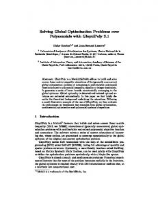
The comparison of single figures of final objective function values and the associated computation times can be totally misleading. In order to provide with a more fair comparison of the different methods, a plot of the convergence curves (objective function values represented as relative error versus computation time) is presented in Fig. 1, where the best three curves per method from a set of 30 are plotted. It can be seen that the ICRS presented the most rapid convergence initially, but was ultimately surpassed by DE and SRES. The latter arrived to the close vicinity of the best known solution much faster then DE, so it could be regarded as the method of choice for this type of problems. 0

10

−1

10

−2

Relative error

10

ICRS GCLSOLVE

−3

10

LJ

−4

DE

10

SRES

−5

10

−6

10

−2

10

0

10

2

10

4

10

6

10

CPU time,s

Fig. 1. Convergence Curves

When solving a global optimization problem, it is usually interesting to examined its multimodal nature. In order to illustrate its non-convexity, the problem was also solved using the multi-start (ms-FMINU) approach, consid-

10

Carmen G. Moles et al.

ering 100 random initial vectors, which were generated satisfying the bounds on the decision variables. This strategy converged to a large number of local solutions, as depicted in the histogram shown in Fig. 2. It is very significant that despite the huge computational effort associated with the 100 runs, the best value found (C ∗ = 23854.71) was still far from the solutions of the GO methods, obtained with much smaller computation times. These results illustrates well the inability of the multi-start approach to handle highly multimodal problems like this one. 18 16 14

Frequency

12 10 8 6 4 2 0 0.5

1

1.5

Objective function

2

2.5 4

x 10

Fig. 2. Histogram of solutions found by the multi-start strategy

Finally, the solutions found were compared with that of Keller et al. [19] by inspecting the decision variables values at the different optima. Plots of the decision variables for the best solutions (i.e. for the DE and SRES algorithms) are presented in Fig. 3 and Fig. 4. It should be noted that there are somewhat significative differences in the optimal abatement and investment policies obtained, although the objective function values are very similar. This indicates a very low sensitivity of the cost function with respect to that control variables, a rather frequent result in dynamic optimization problems.

6 Conclusions In this study, we have shown how a challenging optimal control problem regarding the design of optimal greenhouse gas emissions can be efficiently solved by using several global optimization (GO) methods. Despite the main drawback of stochastic GO methods (i.e., inability to guarantee global optimality), several of these methods were capable of reaching very good solutions in moderate computation times.

Global optimization of climate control problems

11

45

40

DE (f=26398.71) SRES (f=26398.64) Best Solution (f=26398.83)

Abatement (%)

35

30

25

20

15

10

2000

2050

2100

2150

years

Fig. 3. Abatement of CO2 policy (best results of this paper versus best result of Keller et al. (2000) [20]) 20 DE (f=26398.71) SRES (f=26398.64) Best solution (f=26398.83)

Investment (%)

19

18

17

16

2000

2050

years

2100

2150

Fig. 4. Investment policy (best results of this paper versus best result of Keller et al. (2000) [20])

12

Carmen G. Moles et al.

Evolutionary strategies (represented by the SRES method) presented the fastest convergence to the vicinity of the best known solution, closely followed by several other hybrid and stochastic methods. Differential Evolution (DE) arrived to the best solution, although at a rather large computational cost. Simple adaptive stochastic methods were not able to arrive to very refined results, but they presented an interesting first period of fast convergence which suggest new hybrid approaches.

References 1. Ali M, Storey C, T¨ orn A (1997) Application of stochastic global optimization algorithms to practical problems. J. Optim. Theory Appl., 95(3):545–563 2. Balsa-Canto E, Alonso A A, Banga J R (1998) Dynamic optimization of bioprocesses: deterministic and stochastic strategies. Presented at ACoFop IV (Automatic Control of Food and Biological Processes) G¨ oteborg-Sweden., 21-23 September 3. Banga J R, Casares J (1987) ICRS: Application to a wastewater treatment plant model. In I. S. S. 100, editor, Process Optimisation, IChemE Symposium Series No. 100, pages 183–192. Pergamon Press, Oxford, UK 4. Banga J R, Irizarry R, Seider W D (1998) Stochastic optimization for optimal and model-predictive control. Comput. Chem. Eng., 22(4-5):603–612 5. Banga J R, Seider W D (1996) Global optimization of chemical processes using stochastic algorithms. In: State of the Art in Global Optimization, C. A. Floudas and P. M. Pardalos (eds.), Kluwer Academic Pub., Dordrecht, The Netherlands, pages 563–583 6. Boender C, Kan A R, Timmer G, Stougie L (1982) A stochastic method for global optimization. Math. Programming, 22:125 7. Broecker W (2000) Abrupt climate change: Causal constraints provided by the paleoclimate record. Earth-Science Reviews, 51(1-4):137–154 8. Carrasco E, Banga J R (1997) Dynamic optimization of batch reactors using adaptive stochastic algorithms. Ind. Eng. Chem. Res., 36(6):2252–2261 9. Csendes T (1998) Nonlinear parameter estimation by global optimization efficiency and reliability. Acta Cybernetica, 8(4):361–370 10. Goulcher R, Casares J (1978) The solution of steady-state chemical engineering optimisation problems using a random-search algorithm. Comput. Chem. Eng., 2:33–36 11. Grace A (1994) Optimization Toolbox User’s Guide. The Math Works Inc 12. Grossmann I (1996) Global Optimization in Engineering Design. Kluwer Academic Publishers 13. Guus C, Boender E, Romeijn H (1995) Stochastic Methods, chapter In Horst, R. Pardalos, P.M. eds. Handbook of Global Optimization. Kluwer Academic Publishers, R. Horst and P.M. Pardalos edition 14. Holmstr¨ om K (1999) The TOMLAB optimization environment in matlab. Adv. Model. Optim., 1:47 15. Horst R, Tuy H (1990) Global Optimization: Deterministic Approaches. Springer-Verlag, Berlin, Germany 16. Huyer W, Neumaier A (1999) A global optimization by multilevel coordinate search. Journal of Global Optimization, 14:331–355

Global optimization of climate control problems

13

17. Jarvi T (1973) A random search optimiser with an application to a maxmin problem. page 3. Publications of the Inst. of Appl. Math. Univ. of Turk 18. Jones D (2001) DIRECT. In Encyclopedia of Optimization 19. Keller K, Bolker B, Bradford D (2002) Uncertain climate thresholds in economic optimal growth models. Journal of Environmental Economics and Management, in review 20. Keller K, Tan K, Morel F, D.F B (2000) Preserving the ocean circulation: Implications for climate policy. Climatic Change, 47:17–43 21. Luus R, Jaakola T (1973) Optimisation of non-linear functions subject to equality constraints. IEC Process. des. Dev., 12:380–383 22. Nordhaus W (1994) Managing the Global Commons: The Economics of Climate Change. The MIT Press, Cambridge, Massachusetts 23. Pinter J (1996) Global Optimization in Action. Continuous and Lipschitz Optimization: Algorithms, Implementations and Applications. Kluwer Academics Publishers, Dordrecht 24. Rahmstorf S (1997) Risk of the sea-change in the atlantic. Nature, 388:825–826 25. Runarsson T, Yao X (2000) Stochastic ranking for constrained evolutionary optimization. IEEE Transactions on Evolutionary Computation, 4:284–294. 26. Stocker T, Schmittner A (1997) Influence of CO2 emission rates of the stability of the thermohaline circulation. Nature, 388:862–865 27. Storn R, Price K (1997) Differential evolution - a simple and efficient heuristic for global optimization over continuous spaces. Journal of Global Optimization, 11:341–359 28. Tol R, de Vos A (1998) A bayesian statistical analysis of the enhanced greenhouse effect. Climatic Change, 38:87–112 29. T¨ orn A, Ali M, Viitanen S (1999) Stochastic global optimization: Problem classes and solution techniques. Journal of Global Optimization, 14:437