CHAOS 20, 023124 共2010兲
Global stabilization of fixed points using predictive control Eduardo Liz1,a兲 and Daniel Franco2,b兲 1
Departamento de Matemática Aplicada II, E.T.S.I. Telecomunicación, Universidad de Vigo, Campus Marcosende, 36310 Vigo, Spain 2 Departamento de Matemática Aplicada, Universidad Nacional de Educación a Distancia, Apartado de Correos 60149, 28080 Madrid, Spain
共Received 25 November 2009; accepted 3 May 2010; published online 17 June 2010兲 We analyze the global stability properties of some methods of predictive control. We particularly focus on the optimal control function introduced by de Sousa Vieira and Lichtenberg 关Phys. Rev. E 54, 1200 共1996兲兴. We rigorously prove that it is possible to use this method for the global stabilization of a discrete system xn+1 = f共xn兲 into a positive equilibrium for a class of maps commonly used in population dynamics. Moreover, the controlled system is globally stable for all values of the control parameter for which it is locally asymptotically stable. Our study highlights the difficulty of obtaining global stability results for other methods of predictive control, where higher iterations of f are used in the control scheme. © 2010 American Institute of Physics. 关doi:10.1063/1.3432558兴 In many situations, the mechanisms of control of chaos and targeting seek not only to suppress any possible chaotic behavior, leading the system to a suitable equilibrium, but also to make its basin of attraction as large as possible. While local stability analysis is not difficult to address, in general, global stability results are often based on numerical observance. We tackle this problem for some methods of predictive control and succeed in proving a sharp result of global stabilization valid for a wide family of maps usually employed in the mathematical modeling of discrete systems. I. INTRODUCTION
We discuss the issue of global stabilization of a chaotic dynamical system into an equilibrium employing predictionbased control 共PBC兲, that is, techniques for control of chaos that use predicted iterations of the system. As far as we know, these methods were introduced for discrete dynamical systems by Ushio and Yamamoto.1 However, we point out that in the case of stabilization of fixed points, the same method was first suggested by de Sousa Vieira and Lichtenberg;2 using a combination of a nonlinear delayed feedback control 共DFC兲 method3 and a technique of Socolar et al.,4 they arrived at an “optimal” control technique that overcomes some admitted drawbacks of the DFC method. Some interesting generalizations of PBC methods were introduced by Polyak and Maslov.5,6 One of the advantages of predictive control methods is that conditions for local stabilization of fixed points in terms of the control parameter are easy to find.1,2 However, the problem of global stabilization is more difficult to address, and, except for very particular maps,2,7 only conclusions based on simulations can be found in literature so far.5,6 As explained by Bocaletti et al. 共Ref. 8, Sec 4.1兲, when talking a兲
Author to whom correspondence should be addressed. Electronic mail:
[email protected]. URL: http://www.dma.uvigo.es/ eliz. b兲 Electronic mail:
[email protected]. 1054-1500/2010/20共2兲/023124/9/$30.00
about the problem of targeting, in many practical situations, it is important to drive most trajectories of a dynamical system to a periodic orbit that yields superior performance over the others according to some criteria. Thus, the problem of targeting consists not only of choosing an appropriate attractor but also making its basin of attraction as large as possible. Among the dynamical systems exhibiting chaos, a wellknown family is given by one-dimensional maps of the form xn+1 = f共xn兲,
共1兲
where f is a unimodal function with a unique positive equilibrium K. Examples of such maps employed in the modeling of population dynamics are the quadratic map f共x兲 = rx共1 − x兲, the exponential 共Ricker兲 map f共x兲 = xer共1−x兲, and the generalized Beverton–Holt map f共x兲 = rx / 共1 + x␥兲 共see Ref. 9兲. Here, r and ␥ are positive parameters intrinsic to the model, such as the natural growth rate. It is worth noticing that, although these three maps can be considered discrete approximations of the continuous logistic equation, the Ricker and the Beverton–Holt models have more biological meaning 共see, e.g., Ref. 10兲. One important property, shared by these and other models, is that they exhibit chaos for some values of the parameters,11 but multistability is not possible; this means that even if they have an infinite number of periodic orbits, at most one of them can be attracting. In particular, if the unique positive equilibrium K is asymptotically stable 关that is, 兩f ⬘共K兲兩 ⬍ 1兴, then it is a global attractor. A very interesting mathematical derivation of this property is due to Singer,12 who used the Schwarzian derivative as a fundamental tool. In this setting, an important control problem consists of stabilizing the unique positive equilibrium, keeping the global property, that is, in such a way that all positive trajectories converge to the equilibrium. The aim of most of the proposed mechanisms of control of chaos consists of stabilizing one of the unstable periodic orbits 共UPOs兲 embedded in a chaotic attractor either by adjusting a parameter of the model, or modifying the state variable, by introducing an
20, 023124-1
© 2010 American Institute of Physics
023124-2
Chaos 20, 023124 共2010兲
E. Liz and D. Franco
external parameter that one can control to drive the chaotic system to a stable situation. The first strategy has its origin in the seminal work of Ott, Grebogi, and Yorke;13 although it was successfully applied in physics, it is difficult to implement in ecological systems 共for more comments and references, see Ref. 8, Sec. 2兲. The second group of methods seems to be the most appropriate when we try to manage biological systems since intrinsic parameters such as the growth rate are, in general, difficult to modify, while external parameters such as migration, culling, or enrichment are more easily controllable 共for further discussion and references see, e.g., Ref. 14兲. One of the methods suggested in this context is the constant feedback 共CF兲 method,15 which consists of modifying the one-dimensional system 共1兲 to xn+1 = f共xn兲 − C,
共2兲 16
where C is a positive constant. Gueron proved analytically that for a general family of unimodal maps, it is always possible to find values of C for which Eq. 共2兲 has a stable positive equilibrium. However, the region of attraction is usually small and many trajectories are driven to zero. Biologically, this means that only intermediate values of the population size survive after control, while the others go to extinction due to the Allee effect.10,17 The first author recently proved18 a result of global stabilization for the proportional feedback 共PF兲 control method, which modifies Eq. 共1兲 to xn+1 = f共␥xn兲,
共3兲
where ␥ 苸 共0 , 1兲. In population dynamics, this means that a percentage of the population is removed by migration or harvesting. The other interesting strategy of control is based on a threshold mechanism. The idea of incorporating a selfregulatory threshold dynamics on a chaotic system goes back to the work of Sinha and Biswas19 and Glass and Zheng20 共see also Refs. 21 and 22兲. This strategy of control has also a clear interpretation in biological terms, corresponding to control measures such as culling of a stock population, hunting or catching of a managed population stock, or treatment of infectious diseases 共for more comments and further references, see Ref. 23兲. In this paper, we focus on global stabilization of system 共1兲 using predictive feedback control. Methods of predictive control to stabilize an unstable T-periodic orbit of the discrete-time system 共1兲 have the form1 xn+1 = g共xn,un兲, where the control input un is determined by the difference between the predicted state f T共xn兲 and the current state xn, that is, un = f T共xn兲 − xn . As usual, f T is defined as the Tth iteration of f, and it is used as a prediction of xn+T. For T = 1 共stabilization of fixed points兲, the simplest scheme of PBC is written as
xn+1 = f共xn兲 − ␣共f共xn兲 − xn兲,
共4兲
where ␣ is a real control parameter. Equation 共4兲 is exactly the control proposed by de Sousa Vieira and Lichtenberg 共Ref. 2, Sec. III兲 to avoid some handicaps of the DFC method, such as the increase in dimensionality of the system3 and the so-called odd limitation number.24 Some additional good properties of the control law 共4兲 underlined in Ref. 2 are that the fixed points of the controlled system are the same as those in the uncontrolled system, knowledge of the location of the UPO is not necessary, and it is easy to implement in the sense that the control term contains only the amplified versions of the input and output of the dynamical system. In our main result, we prove that for a family of unimodal maps, including the quadratic map, the Ricker map, and the generalized Beverton–Holt map, the optimal nonlinear control of de Sousa Vieira and Lichtenberg leads to the global stabilization of a chaotic system into its positive equilibrium. Moreover, this is true for all values of the parameters for which local stabilization is possible. We also discuss the case of more general methods of predictive control, showing that this result of global stability is no longer valid. This paper is organized as follows: in Sec. II, we state our main assumptions and recall some related results. Section III is devoted to establish the main global stability result. In Sec. IV, the issue of local and global stability is discussed for other PBC methods. Finally, in Sec. V, we discuss the main conclusions and directions for future research. The proofs and auxiliary results are placed in Appendixes A and B. II. STATEMENT OF THE PROBLEM
First, we introduce some general properties and notation that will be used throughout the paper from now on. Denote by I = 关0 , b兴 a real interval 共b = +⬁ is allowed兲. The map f : I → I that defines the dynamical system 共1兲 will be a C3 function satisfying the following properties: 共A1兲 f has only two fixed points: x = 0 and x = K ⬎ 0, with f ⬘共0兲 ⬎ 1. 共A2兲 f has a unique critical point c ⬍ K in such a way that f ⬘共x兲 ⬎ 0 for all x 苸 共0 , c兲, f ⬘共x兲 ⬍ 0 for all x 苸 共c , b兲. 共A3兲 共Sf兲共x兲 ⬍ 0 for all x ⫽ c, where 共Sf兲共x兲 =
冉 冊
f 共x兲 3 f ⬙共x兲 − f ⬘共x兲 2 f ⬘共x兲
2
is the Schwarzian derivative of f. 共A4兲 f ⬙共x兲 ⬍ 0 for all x 苸 共0 , c兲. These assumptions are motivated by the fact that many maps usually employed in discrete models fulfill them. In particular, the quadratic map for all r ⬎ 1, the exponential map for all r ⬎ 0, and the generalized Beverton–Holt map for r ⬎ 1 and ␥ ⱖ 2 共see Ref. 12兲. We notice that if f satisfies 共A3兲 and f ⬙共0兲 ⬍ 0, then condition 共A4兲 holds; otherwise, f ⬘ would have a positive local minimum, which contradicts the maximum principle 共Ref. 12, Proposition 2.4兲. Thus, the family of maps satisfying conditions 共A1兲–共A4兲 is essentially
023124-3
Chaos 20, 023124 共2010兲
Global stabilization
1.0 0.8 0.6 0.4 0.2 0.0
0.0
0.2
0.4
0.6
0.8
1.0
FIG. 1. 共Color online兲 Graph of the map f共x兲 = 4x2共1 − x兲 and the line y = x. The iterates of initial points x0 ⬍ 1 / 2 converge to zero 共Allee effect兲.
the family of S-unimodal maps considered by Collet and Eckmann 共Ref. 25, Sec. II.4兲 共see also Ref. 26, Sec. 5.3兲. Similar conditions were assumed for CF control in Refs. 16 and 17 and for PF in Ref. 18. Besides the above-mentioned maps, there are other functions satisfying conditions 共A1兲– 共A4兲, which do not come from population dynamics; an example is the sine map f共x兲 = r sin共x兲, 0 ⱕ x ⱕ 1, with r 苸 共1 / , 1兲 共Ref. 27, p. 369兲. When used in population models, maps satisfying condition 共A4兲 correspond to compensation models, where the per capita production is a decreasing function of the population density 关see, e.g., Ref. 28 共Sec. 1.2兲 and Ref. 29 共Sec. 1.4兲兴. This condition is not satisfied by depensation models, for which the per capita production is smaller than one for low values of the population density. The latter models exhibit the so-called Allee effect, which means that if the initial population size is below a critical parameter, the population will die out. An example is the generalization of the quadratic map f共x兲 = rx2共1 − x兲 共see Ref. 28兲. In Fig. 1, we plot the graph of this map with r = 4; although it has a unique positive fixed point and a unique critical point 共maximum兲, it does not satisfy 共A4兲 and exhibits the Allee effect. Condition 共A3兲 is a more technical assumption. The Schwarzian derivative was first introduced into the study of one-dimensional dynamical systems by Singer,12 and it became a valuable tool 共see, e.g., Refs. 25 and 26兲. Although it is difficult to give a biological interpretation of it, it is a remarkable fact 共already observed by Singer兲 that the most usual maps employed in the modeling of population dynamics satisfy condition 共A3兲. We recall12 that if f satisfies conditions 共A1兲 and 共A3兲, and f ⬘共K兲 ⱖ −1, then K is a global attractor of system 共1兲. We notice that, for ␣ 苸 关0 , 1兴, the method 共4兲 is welldefined in the sense that, since f : I → I, the modified map F␣共x兲 ª f共x兲 − ␣共f共x兲 − x兲 = ␣x + 共1 − ␣兲f共x兲 also maps I into I because F␣共x兲 is a convex combination of x and f共x兲. This property does not hold for general DFC and PBC methods. If we think of population models, this is important because negative values of the population do not make sense. We limit our discussion to this range of values of the control parameter ␣.
The method 共4兲 was applied in Ref. 2 to the quadratic map, with r ⬎ 3 关to ensure that K is unstable for f共x兲 = rx共1 − x兲兴. The authors observed that the positive fixed point K = 1 − 1 / r is locally stable for the controlled system if ␣ ⬎ 共r − 3兲 / 共r − 1兲 ª ␣0. Moreover, the equilibrium K is a global attractor for system 共4兲 for all ␣ 苸 共␣0 , 1兲. However, as pointed out later by McGuire et al.,7 the quadratic map is a very particular case since the modified map F␣ is still quadratic. Hence, it trivially shares the global stability properties of f. For general unimodal maps, function F␣ does not inherit properties 共A2兲 and 共A3兲; usually, the shape of F␣ is no longer one-humped for ␣ ⬎ 0. For example, the exponential map f共x兲 = xer共1−x兲 is bimodal for 0 ⬍ ␣ ⬍ er−2 / 共1 + er−2兲 and increasing for er−2 / 共1 + er−2兲 ⬍ ␣ ⬍ 1.30 Thus, although numerical experiments suggest that K is still globally attracting for F␣ when 兩F␣⬘ 共K兲兩 ⬍ 1, an analytic proof of this result is not available. Our main result in this paper fills this gap for the family of maps satisfying conditions 共A1兲–共A4兲. III. GLOBAL STABILIZATION
In this section, we state our main result. As before, we denote F␣共x兲 = ␣x + 共1 − ␣兲f共x兲. We begin with a preliminary result, which is of independent interest. Proposition 1: Assume that f ⬘共x兲 ⬍ 0 and F␣⬘ 共x兲 ⬍ 0 for all x in an interval J 傺 I. If 共Sf兲共x兲 ⬍ 0 for all x 苸 J, then 共SF␣兲共x兲 ⬍ 0 for all x 苸 J and all ␣ 苸 共0 , 1兲. As an immediate consequence of Proposition 1 and Theorem 5 in Ref. 31, we get the following corollary. Corollary 1: If f satisfies conditions (A1)–(A3), and f ⬘共K兲 ⬍ −1, then the family of maps 兵F␣ : ␣ 苸 共0 , 1兲其 undergoes a period-doubling bifurcation at ␣0 = 共f ⬘共K兲 + 1兲 / 共f ⬘共K兲 − 1兲, where F␣⬘ 共K兲 = −1. 0 Corollary 1 solves an open problem posed in Ref. 7. There, the authors proposed to investigate the conditions under which period doubling occurs for general unimodal maps, which are being stabilized at a fixed point using control 共4兲. They showed that if f has a negative Schwarzian derivative, then the same property is inherited by F␣ when the positive feedback parameter ␣ is sufficiently small. Corollary 1 proves that period doubling occurs regardless of the value of ␣ 苸 共0 , 1兲 necessary for stabilization. Next we formulate our main result. Theorem 1: Assume that f satisfies conditions (A1)–A4), and define F␣共x兲 = f共x兲 − ␣共f共x兲 − x兲. If F␣⬘ 共K兲 ⱖ −1, then the positive equilibrium K is a global attractor of Eq. (4) on 共0 , b兲. The proofs of Proposition 1 and Theorem 1 can be found in Appendix A. As an example, consider the Ricker map f共x兲 = xer共1−x兲, which satisfies conditions 共A1兲–共A4兲 for all r ⬎ 0. The positive equilibrium K = 1 is globally stable for r ⱕ 2, then it undergoes a typical sequence of period-doubling bifurcations, and it becomes chaotic for r ⬎ 2.6924.11 According to Corollary 1 and Theorem 1, for all r ⬎ 2, the family of maps 兵F␣共x兲 = ␣x + 共1 − ␣兲xer共1−x兲 : ␣ 苸 关0 , 1兲其
023124-4
Chaos 20, 023124 共2010兲
E. Liz and D. Franco
n=0
2.5
2.5
2.0
xn
2.0
1.5
1.5
1.0
1.0
0.5
0.0
0.5 0.0
0.1
0.2
α
0.3
1/3
0.4
FIG. 2. 共Color online兲 Bifurcation diagram for the controlled system 共5兲 with r = 3 and ␣ as the bifurcation parameter. The value ␣ = 0 corresponds to the uncontrolled 共chaotic兲 system; the equilibrium becomes globally asymptotically stable after the bifurcation point ␣ = 1 / 3 共vertical dashed line兲.
experiences a period-halving bifurcation at ␣ = 共r − 2兲 / r in such a way that the positive equilibrium is globally attracting for the controlled system xn+1 = xner共1−xn兲 − ␣共xner共1−xn兲 − xn兲
共5兲
for all ␣ 苸 关共r − 2兲 / r , 1兲. We show the bifurcation diagram for r = 3 in Fig. 2. The equilibrium is stabilized in a periodhalving bifurcation at ␣ = 1 / 3 共see the vertical dashed line兲. Theorem 1 ensures that, for ␣ ⱖ 1 / 3, all orbits starting at x0 ⬎ 0 converge to the positive equilibrium K = 1. Next we give a numerical validation of Theorem 1 by means of a statistical approach applied to Eq. 共5兲 with r = 3; this method not only illustrates our main result but also provides significant rates of convergence, not dependent on the initial condition. First we choose randomly 2000 initial conditions in the interval 关0,2.5兴, which is invariant and attracting for the map f. See Fig. 3, where we show the distribution of this sample and its evolution after 15 iterations of f. Since the uncontrolled system is chaotic, no periodic pattern is appreciated. We notice that, in Figs. 3–8, n denotes the number of iterations. Figure 4 shows the distribution of the random sample after 15 iterations of the controlled system for ␣ = 0.35, which is close to the bifurcation point. It can be observed that the iterates of all initial conditions approach the positive equilibrium. The convergence is faster for larger values of ␣, as it is shown for ␣ = 0.4 and the same number of iterations. Next we estimate the probability density function of the random variable provided by the sample we chose using a kernel density estimation. We use the kernel density approximation m
冉 冊
1 x − xi 共x兲 = k , 兺 hm i=1 h m where 共xi兲i=1 is the sample, k is the standard Gaussian function
500
1000
1500
2000
1500
2000
(a)
α=0, n=15 2.5
2.0
1.5
1.0
0.5
0
500
1000
(b) FIG. 3. 共Color online兲 Distribution of a sample of 2000 random initial conditions in the interval 关0,2.5兴, and the evolution of the uncontrolled system 共␣ = 0兲 after 15 iterations.
k
冉 冊
1 −共x − x 兲2/2h2 x − xi i = , 冑2 e h
and h is a smoothing bandwidth. We use
冉
m
m
h = max兵xi其 − min兵xi其 i=1
i=1
冊冒
4.
Our simulations with different samples of random initial conditions show that, when evolved under the equations of the controlled system 共5兲, the approximation of the probability density function converges to a delta function located at the positive fixed point. In Fig. 5, we represent the initial density function and its evolution after 50 iterations of the uncontrolled system 关Eq. 共5兲 with ␣ = 0兴. As observed before, there is no periodic pattern. The evolution of the density function for ␣ = 0.35 共close to the bifurcation point ␣ = 1 / 3兲 after 15 and 50 iterations is shown in Fig. 6. The convergence to the delta function is faster for larger values of ␣, as shown in Fig. 7 for ␣ = 0.4: after only 15 iterations, the density function is highly concentrated at the positive equilibrium point K = 1.
023124-5
Chaos 20, 023124 共2010兲
Global stabilization
α=0.35, n=15
n=0
φ(x)
2.5
2.0
0.3
1.5
0.2
1.0
0.1
0.5 0.5
1.0
(a) 0
500
1000
1500
2000
(a)
α=0.4, n=15
x
1.5
2.0
2.5
2.0
2.5
α=0, n=50
φ(x) 0.35
2.5
0.30 0.25
2.0
0.20 0.15
1.5
0.10
1.0
0.05
0.5
0.5
(b)
0
500
1000
1500
2000
(b)
1.0
x
1.5
FIG. 5. 共Color online兲 Approximation of the probability density function for the random variable corresponding to a sample of 2000 random initial conditions in the interval 关0,2.5兴, and its evolution after 50 iterations under the uncontrolled system 共5兲 with r = 3 and ␣ = 0.
FIG. 4. 共Color online兲 Evolution of the random sample of 2000 initial conditions in the interval 关0,2.5兴 after 15 iterations of the controlled system for ␣ = 0.35 and ␣ = 0.4.
xn+1 = f共xn兲 + 共− 1兲m+1共f m+1共xn兲 − f m共xn兲兲, To further illustrate this numerical validation, we show in Fig. 8 the time series of the solution of Eq. 共5兲, with r = 3 and initial point x0 = 0.5, for ␣ = 0.35 and ␣ = 0.4.
IV. OTHER METHODS OF PREDICTIVE CONTROL
The global control attained with the method of de Sousa Vieira and Lichtenberg has the restriction that, in general, the perturbation required to stabilize all trajectories around the positive equilibrium is relatively large. In this regard, we emphasize that, while targeting problems usually require small perturbations, there are situations where large perturbations are more appropriate. For example, this is the case of interventions in population dynamics, where the control problem can be seen as a strategy for sustainable development 共e.g., by culling or enrichment兲.14,23,32,33 In order to reduce the control perturbation, an interesting generalization of PBC methods was introduced by Polyak and Maslov.5,6 Their main idea consists of using higher iterations of the map f as predicted states. To stabilize a fixed point, this method has the form
共6兲
where m is a positive integer and ⬎ 0. Notice that the case m = 0 is equivalent to Eq. 共4兲, with the usual notation f 0共x兲 ª x. Now, assume that f is a map satisfying conditions 共A1兲– 共A4兲 and K is an unstable equilibrium of Eq. 共1兲. Then, f ⬘共K兲 ⬍ −1, and it is easy to check that K is asymptotically stable for Eq. 共6兲 if ⬎
冉 冊 −1 f ⬘共K兲
m
f ⬘共K兲 + 1 ª m . f ⬘共K兲 − 1
Then, the bifurcation point ␣0 defined in the statement of Corollary 1 for Eq. 共4兲 is replaced by m = 共−1 / f ⬘共K兲兲m␣0 when control 共6兲 is applied. For example, for the chaotic exponential map f共x兲 = xe3共1−x兲, we have f ⬘共K兲 = 2 and ␣0 = 1 / 3. Thus, m = ␣0 / 2m, which means that the perturbation of f in Eq. 共6兲 can be made as small as desired, choosing a sufficiently big value of m. Some disadvantages of this control method are that 共a兲 it is computationally more expensive than Eq. 共4兲, especially for large m, and 共b兲 it is not ensured 共see the example below兲 that the modified map
023124-6
Chaos 20, 023124 共2010兲
E. Liz and D. Franco
α=0.35, n=15
φ(x)
α=0.4, n=5
φ(x) 3.5
4
3.0 2.5
3
2.0 2
1.5 1.0
1
0.5 0.5
(a)
1.0
x
1.5
2.0
2.5
α=0.35, n=50
φ(x)
1.0
x
1.5
2.0
2.5
2.0
2.5
α=0.4, n=15
φ(x)
30
(b)
0.5
(a)
30
25
25
20
20
15
15
10
10
5
5
0.5
1.0
x
1.5
2.0
2.5
FIG. 6. 共Color online兲 Evolution of the approximation of the probability density function for the random variable corresponding to a sample of 2000 random initial conditions in the interval 关0,2.5兴 after 15 and 50 iterations under the controlled system 共5兲 with r = 3 and ␣ = 0.35.
F,m共x兲 = f共x兲 + 共− 1兲m+1共f m+1共x兲 − f m共x兲兲 is well-defined for m ⱖ 2. We notice that the scheme for m = 1 is still well-defined for 苸 关0 , 1兴 because F,1共x兲 = f共x兲 + 共f 2共x兲 − f共x兲兲 = 共1 − 兲f共x兲 + f 2共x兲 is a convex combination of f共x兲 and f 2共x兲. A natural question is whether or not the global stability result valid for m = 0 still holds for Eq. 共6兲 when m ⬎ 0. In Ref. 6, it is claimed that this is an expected property, confirmed by simulation results using the quadratic family. However, we show that, in general, the asymptotic stability of the equilibrium is only a local property. Indeed, even when the equilibrium is locally stable, system 共6兲 can have other stable periodic orbits, including new fixed points. For example, for m = 2 and the chaotic quadratic map f共x兲 = 3.9x共1 − x兲, the fixed point K = 0.7435 is locally stable for Eq. 共6兲 when ⬎ 2 = 0.086. However, for any arbitrarily close to 2, there is a new fixed point K1 in such a way that all orbits starting at a point x0 ⬍ K1 converge to zero. This means that the control method induces an Allee effect. In Fig. 9共a兲, we plot the function F,2共x兲 = f共x兲 − 共f 3共x兲 − f 2共x兲兲, with = 0.1 共solid line兲; for the sake of comparison, we also include the graph of function f共x兲 = 3.9x共1 − x兲 corresponding
(b)
0.5
1.0
x
1.5
FIG. 7. 共Color online兲 Evolution of the approximation of the probability density function for the random variable corresponding to a sample of 2000 random initial conditions in the interval 关0,2.5兴 after 5 and 15 iterations under the controlled system 共5兲 with r = 3 and ␣ = 0.4.
to the uncontrolled system 共dashed line兲 and the line y = x. A magnification of the graph of F,2 between 0 and 0.05 is included in Fig. 9共b兲 to emphasize the new positive fixed point K1 ⬇ 0.016 06 and the Allee effect. In Appendix B, we prove that a global stability result holds for m = 1 in Eq. 共6兲 when f is the quadratic map, but this is an exception. In general, even for m = 1, the conclusions of Corollary 1 and Theorem 1 are no longer valid. Consider m = 1 in Eq. 共6兲, that is, xn+1 = f共xn兲 + 共f 2共xn兲 − f共xn兲兲,
共7兲
with f共x兲 = xe3共1−x兲. The family of maps F,1共x兲 = f共x兲 + 共f 2共x兲 − f共x兲兲 undergoes a period-doubling bifurcation at = 1 / 6 ⬇ 0.166, where F,1 ⬘ 共1兲 = −1. The fixed point K = 1 is locally stable for ⬎ 1 / 6, but this equilibrium coexists with an attracting 2-cycle until this cycle disappears in a tangent bifurcation at ⬇ 0.1958. After this value, the positive fixed point seems to be globally attracting, but only until a new fixed point appears at ⬇ 0.4605. In Fig. 10, we show the bifurcation diagram for 苸 关0 , 0.3兴. The unstable fixed point is represented by a dashed line between = 0 and = 1 / 6. The other dashed lines represent an unstable 2-cycle that disappears 共with the attracting 2-cycle兲 after a saddle-node bifurcation at ⬇ 0.1958.
023124-7
Chaos 20, 023124 共2010兲
Global stabilization
α=0.35 1.6
0.8
1.4
xn
(a)
1.0
1.2
0.6
1.0
0.4
0.8 0.6 0.4
0.2 0
10
20
(a)
30
n
40
50
60
α=0.4
0.0
0.0
0.2
0.4
0.6
0.8
1.0
0.03
0.04
0.05
(b)
0.05
1.6
0.04
1.4
0.03
1.2
xn 1.0
0.02
0.8
0.01
0.6 0.4
(b)
0.00 0
10
20
30
n
40
50
60
FIG. 8. 共Color online兲 Time series for the controlled system 共5兲 with r = 3; the values of the control parameter are ␣ = 0.35 and ␣ = 0.4. In both cases, the initial point is x0 = 0.5, and 60 iterations were made.
V. CONCLUSIONS AND DIRECTIONS FOR FUTURE RESEARCH
We have analyzed the global stability properties of some methods of predictive control. We particularly focused on the optimal control function introduced by de Sousa Vieira and Lichtenberg.2 Based on their analysis of the logistic map, they affirmed that this method has good global stabilizing properties, thus decreasing the sensitivity to noise. Our main result 共Theorem 1兲 comes up with a rigorous analytic proof of this observation for a family of maps commonly used in modeling of discrete-time systems. Moreover, we have given a positive answer to some questions related to the preservation of the period-doubling route to chaos in the controlled system posed in Ref. 7. We have reviewed as well the local and global properties of stabilization of fixed points of more general PBC methods. An important property of these methods is that they do not increase the dimension of the system; thus, the study of local stability is easier than in other control techniques. However, our study highlights the difficulty of obtaining global stability results when using higher iterations of the map f in the control scheme. de Sousa Vieira and Lichtenberg proposed a generalization of their optimal method to stabilize UPOs with prime period T ⬎ 1 by using the map F␣,T共x兲 = f T共x兲 − ␣共f T共x兲 − x兲. Assume that we aim to stabilize an UPO of period T = 2m of
0.00
0.01
K1
0.02
FIG. 9. 共Color online兲 共a兲 Graphs of functions f共x兲 = 3.9x共1 − x兲 共dashed line兲 and F,2共x兲 = f共x兲 − 共f 3共x兲 − f 2共x兲兲, with = 0.1 共solid line兲. The fixed points are obtained as the intersections with the line y = x. 共b兲 Magnification of the graph of F,2 between 0 and 0.05; the fixed point K1 ⬇ 0.016 06 induces an Allee effect: all initial conditions below K1 are driven to zero under successive iterations of F,2.
a chaotic map f using this method. An interesting problem to study is whether or not it is possible to get a globally stable T-periodic orbit in the sense that it attracts all initial conditions, which are not an element of the other UPOs. Numerical simulations suggest that this is true for T = 2 and f satis-
2.5 2.0
xn
1.5 1.0 0.5 0.0 0.00
0.05
0.10
0.15
ε
0.20
0.25
0.30
FIG. 10. 共Color online兲 Bifurcation diagram for the controlled system 共7兲 with f共x兲 = xe3共1−x兲 and as the bifurcation parameter. The fixed point K = 1 is locally asymptotically stable but not globally stable between 0.166 and 0.1958. The dashed lines indicate instability.
023124-8
Chaos 20, 023124 共2010兲
E. Liz and D. Franco
fying conditions 共A1兲–共A4兲; to find a proof of this result would be a nice improvement of Theorem 1. However, the answer to this problem is, in general, negative for T ⬎ 2. For example, the quadratic map f共x兲 = 4x共1 − x兲 has two distinct four-periodic orbits with the same multiplier = −16; thus, global stabilization of one of them is not possible with this control scheme. An additional application of the new results proved in this paper is that the controlled map F␣共x兲 = ␣x + 共1 − ␣兲f共x兲 is used as a model in population dynamics when a probability of surviving the reproductive season 共iteroparous populations兲 is assumed. If f means the nonlinear density growth of the population, the model xn+1 = F␣共xn兲 = ␣xn + 共1 − ␣兲f共xn兲
共8兲
assumes that a fraction ␣ of energy is invested into adult survivorship rather than reproduction 共for more details, see Refs. 10 and 30兲. Thus, Theorem 1 shows that even if f is chaotic and the survivorship parameter ␣ is large enough, the population is stabilized into the positive equilibrium regardless the initial size of the population. We notice that organisms might evolve into such strategy 共survival rather than reproduction兲 under bad environmental conditions; this means that a population whose fecundity encodes for chaos can stabilize itself at its equilibrium density. For a nice discussion on the evolutionary advantage of self-control, see Ref. 34. As stated there, this makes a difference between ecological systems and physical or chemical systems. Regarding the application of PBC methods to population problems, an important drawback is that their implementation requires full knowledge of the model equation. Although the exact form of the original map is difficult to obtain, in some cases good census data are available 共see, e.g., Ref. 35, where census data of a freshwater fish population were collected every fourth month over 20 years兲; this allows one to derive a stock-recruitment relationship that fits well into some known function, such as the Ricker map. Then, the model can be validated, and the control method could be implemented to stabilize the population. On the other hand, while another admitted drawback in the application of predictive control in the process industries is that a quick computation upon observation must be performed 共see, e.g., Ref. 36兲, in the setting of population dynamics, the time scales are different; for instance, in a fish farm, the control 共4兲 can provide an assessment on whether next season harvesting should be incremented or, conversely, some enrichment is needed to stabilize the stock size. We mention that the control method 共4兲 can help not only to stabilize the population but also to avoid extinction 共see Ref. 30兲. For further discussion and references on the application of control methods to population problems, especially to prevent extinction, we refer to Ref. 33. Related results on global stability in Eq. 共8兲 for particular choices of f were proved in Refs. 37 and 38. ACKNOWLEDGMENTS
The authors sincerely thank the insightful critique of three anonymous reviewers of this paper, which significantly
helped to improve it. We are greatly indebted to Dr. János Karsai from the University of Szeged 共Hungary兲 for very helpful discussions. This research was supported in part by the Spanish Ministry of Science and Innovation and FEDER 共Grant No. MTM2007-60679兲. APPENDIX A: PROOF OF THE MAIN RESULT
Proof of Proposition 1: Since f ⬘共x兲 ⬍ 0 and 共Sf兲共x兲 ⬍ 0 for all x 苸 J, we have 2
冉 冊
f ⬙共x兲 f 共x兲 ⬍3 f ⬘共x兲 f ⬘共x兲
2
⇒ 2f 共x兲 ⬎ 3
共f ⬙共x兲兲2 f ⬘共x兲
for all x 苸 J. Using that F␣⬘ 共x兲 ⬍ 0 on J, the previous inequality, and the obvious relations F␣⬘ 共x兲 = ␣ + 共1 − ␣兲f ⬘共x兲,
F␣⬙ 共x兲 = 共1 − ␣兲f ⬙共x兲,
F␣共x兲 = 共1 − ␣兲f 共x兲, we get, for all x 苸 J, 2F␣共x兲 = 2共1 − ␣兲f 共x兲 ⬎ 3共1 − ␣兲 =3
共F␣⬙ 共x兲兲2
F␣⬘ 共x兲 − ␣
⬎3
共F␣⬙ 共x兲兲2 F␣⬘ 共x兲
共f ⬙共x兲兲2 f ⬘共x兲
.
This inequality implies that 共SF␣兲共x兲 ⬍ 0. To use Proposition 1 to prove our main result, we need the following auxiliary result from Ref. 39. Lemma 1: (Reference 39, Corollary 2.9) Let g : 共0 , b兲 → 关0 , b兴 be a continuous map with a unique fixed point K such that 共g共x兲 − x兲共x − K兲 ⬍ 0 for all x ⫽ K. Assume that there are points 0 ⱕ a ⬍ K ⬍ d ⱕ b such that the restriction of g to 共a , d兲 has at most one turning point and (whenever it makes sense) g共x兲 ⱕ g共a兲 for every x ⱕ a and g共x兲 ⱖ g共d兲 for every x ⱖ d. If g is decreasing at K, assume additionally that 共Sg兲 ⫻共x兲 ⬍ 0 for all x 苸 共a , d兲 except at most one critical point of g, and −1 ⱕ g⬘共K兲 ⬍ 0. Then K is a global attractor of g. Proof of Theorem 1: Notice that f ⬘共0兲 ⬎ 1 implies that F␣⬘ 共0兲 ⬎ 1 for all ␣ 苸 关0 , 1兲. On the other hand, F␣⬘ 共x兲 = 0 ⇔ f ⬘共x兲 = −␣ / 共1 − ␣兲. If F␣ has no critical points, then it is strictly increasing, and therefore K is a global attractor because F␣共x兲 ⬎ x for x 苸 共0 , K兲 and F␣共x兲 ⬍ x for x 苸 共K , b兲. Notice that this happens when f ⬘共x兲 ⬎ −␣ / 共1 − ␣兲 for all x 苸 共0 , b兲. Next, since 共Sf兲共x兲 ⬍ 0 for all x ⫽ c, f can have at most one inflexion point in 共c , b兲. First we consider the case when f has no inflexion points in 共c , b兲. Then f ⬘ is strictly decreasing in 共c , b兲, and there is at most one point c1 ⬎ c such that F␣⬘ 共c1兲 = 0. Clearly, c1 is a local maximum of F␣ since F␣⬘ 共x兲 ⬎ 0 on 共0 , c1兲 and F␣⬘ 共x兲 ⬍ 0 on 共c1 , b兲. If c1 ⬎ K, then F␣⬘ 共K兲 ⬎ 0, and it follows that K is globally attracting. Thus, we can assume that c ⬍ c1 ⬍ K. Since F␣共x兲 ⱕ F␣共c1兲 for all x 苸 共0 , c1兴 and, by Proposition 1, 共SF␣兲共x兲 ⬍ 0 on 共c1 , b兲, an application of Lemma 1 with a = c1, d = b proves that K is a global attractor of F␣. It remains to consider the case when f has an inflexion point ␥ in 共c , b兲. It is clear that f ⬘ attains a global minimum
023124-9
at f ⬘共␥兲. If f ⬘共␥兲 ⱖ −␣ / 共1 − ␣兲, then F␣ is strictly increasing, and therefore, K is a global attractor. Thus, we assume that f ⬘共␥兲 ⬍ −␣ / 共1 − ␣兲. In this case, there are at least one, and at most two critical points c1 ⬍ ␥ ⬍ c2 of F␣. If there is only one, it is a local maximum, and this case is solved as the previous one. If there are two critical points, then F␣ is increasing on 共0 , c1兲 艛 共c2 , b兲 and decreasing on 共c1 , c2兲. Thus, we can apply again Lemma 1, with a = c1, d = c2. The proof is complete. APPENDIX B: GLOBAL STABILIZATION FOR THE QUADRATIC MAP
Consider the quadratic map f共x兲 = rx共1 − x兲; f maps the interval 关0,1兴 into itself if 0 ⱕ r ⱕ 4. It is well known that the positive fixed point K = 1 − 1 / r is globally stable for 1 ⬍ r ⱕ 3 and unstable for r ⬎ 3. Here, we only consider the unstable case. Proposition 2: The PBC scheme (7) stabilizes locally the positive equilibrium of f共x兲 = rx共1 − x兲 for all ⬎ 1共r兲 = 共r − 3兲 / 共r2 − 3r + 2兲. Moreover, K is a global attractor on 关0,1兴 for all 苸 共1共r兲 , 2共r兲兲, where 2共r兲 = 4 / 共r − 1兲2. Proof: As mentioned in Sec. IV, the modified map F共x兲 = f共x兲 + 共f 2共x兲 − f共x兲兲 maps 关0,1兴 into 关0,1兴, and K is asymptotically stable for the controlled system if ⬎ 1共r兲. Moreover, it is easy to check that K = 1 − 1 / r is the unique positive fixed point of F if and only if ⬍ 2共r兲 = 4 / 共r − 1兲2. In order to apply Lemma 1, we first prove that 共SF兲共x兲 ⬍ 0 for all noncritical points of F. Indeed, notice that F共x兲 = 共H ⴰ f兲共x兲, where H共x兲 = x + 共f共x兲 − x兲. Since f and H are quadratic maps, they have a negative Schwarzian derivative. Thus, the result follows from the composition rule 共S共H ⴰ f兲兲共x兲 = 共SH兲共f共x兲兲共f ⬘共x兲兲2 + 共Sf兲共x兲 共see, e.g., Ref. 12, Theorem 2.1兲. Next, observe that F has either only the critical point c = 1 / 2 共local maximum兲 or three critical points c1 ⬍ c ⬍ c2; in the latest case, F共c兲 is a local minimum and F共c1兲 = F共c2兲 are local maxima. If there is only one critical point, the result follows from Singer’s theorem since F is unimodal. If there are three critical points, we complete the proof, applying Lemma 1 to the interval 共a , d兲 = 共c2 , 1兲 if K ⬎ c2 or to the interval 共a , d兲 = 共c1 , c2兲 if K ⬍ c2. T. Ushio and S. Yamamoto, Phys. Lett. A 264, 30 共1999兲. M. de Sousa Vieira and A. J. Lichtenberg, Phys. Rev. E 54, 1200 共1996兲. 3 K. Pyragas, Phys. Lett. A 170, 421 共1992兲. 1 2
Chaos 20, 023124 共2010兲
Global stabilization 4
J. E. S. Socolar, D. W. Sukow, and D. J. Gauthier, Phys. Rev. E 50, 3245 共1994兲. 5 B. T. Polyak, Autom. Remote Control 共Engl. Transl.兲 66, 1791 共2005兲. 6 B. T. Polyak and V. P. Maslov, “Controlling chaos by predictive control,” in Proceedings of the 16th World Congress of IFAC, Praha, 2005. 7 J. McGuire, M. T. Batchelor, and B. Davies, Phys. Lett. A 233, 361 共1997兲. 8 S. Boccaletti, C. Grebogi, Y.-C. Lai, H. Mancini, and D. Maza, Phys. Rep. 329, 103 共2000兲. 9 T. S. Bellows, J. Anim. Ecol. 50, 139 共1981兲. 10 H. R. Thieme, Mathematics in Population Biology, Princeton Series in Theoretical and Computational Biology 共Princeton University Press, Princeton, 2003兲. 11 R. M. May, Nature 共London兲 261, 459 共1976兲. 12 D. Singer, SIAM J. Appl. Math. 35, 260 共1978兲. 13 E. Ott, C. Grebogi, and J. A. Yorke, Phys. Rev. Lett. 64, 1196 共1990兲. 14 R. V. Solé, J. G. P. Gamarra, M. Ginovart, and D. López, Bull. Math. Biol. 61, 1187 共1999兲. 15 S. Parthasarathy and S. Sinha, Phys. Rev. E 51, 6239 共1995兲. 16 S. Gueron, Phys. Rev. E 57, 3645 共1998兲. 17 S. J. Schreiber, J. Math. Biol. 42, 239 共2001兲. 18 E. Liz, Phys. Lett. A 374, 725 共2010兲. 19 S. Sinha and D. Biswas, Phys. Rev. Lett. 71, 2010 共1993兲. 20 L. Glass and W. Zeng, Int. J. Bifurcation Chaos Appl. Sci. Eng. 4, 1061 共1994兲. 21 S. Sinha, Phys. Rev. E 49, 4832 共1994兲. 22 S. Sinha, Phys. Rev. E 63, 036212 共2001兲. 23 F. M. Hilker and F. H. Westerhoff, Phys. Rev. E 73, 052901 共2006兲. 24 T. Ushio, IEEE Trans. Circuits Syst., I: Fundam. Theory Appl. 43, 815 共1996兲. 25 P. Collet and J. P. Eckmann, Iterated Maps on the Interval as Dynamical Systems, Progress in Physics 共Birkhäuser, Boston, 1980兲. 26 A. N. Sharkovsky, S. F. Kolyada, A. G. Sivak, and V. V. Fedorenko, Dynamics of One-Dimensional Maps, Mathematics and Its Applications 共Kluwer Academic, Dordrecht, 1997兲. 27 S. H. Strogatz, Nonlinear Dynamics and Chaos, Studies in Nonlinearity 共Westview, Cambridge, 1994兲. 28 C. W. Clark, Mathematical Bioeconomics, Pure and Applied Mathematics, 2nd ed. 共Wiley, New York, 1990兲. 29 F. Brauer and C. Castillo-Chávez, Mathematical Models in Population Biology and Epidemiology, Texts in Applied Mathematics 共SpringerVerlag, New York, 2001兲. 30 E. Liz, “Complex dynamics of survival and extinction in simple population models with harvesting,” Theor. Ecol. 共2009兲. 31 H. A. El-Morshedy, V. Jiménez López, and E. Liz, Nonlinear Anal.: Real World Appl. 9, 776 共2008兲. 32 F. M. Hilker and F. H. Westerhoff, Phys. Lett. A 362, 407 共2007兲. 33 F. M. Hilker and F. H. Westerhoff, Am. Nat. 170, 232 共2007兲. 34 M. Doebeli, Philos. Trans. R. Soc. London, Ser. B 254, 281 共1993兲. 35 J. Lobón-Cerviá, Can. J. Fish. Aquat. Sci. 64, 1429 共2007兲. 36 D. Q. Mayne, J. B. Rawlings, C. V. Rao, and P. O. M. Scokaert, Automatica 36, 789 共2000兲. 37 E. Liz, Discrete Contin. Dyn. Syst., Ser. B 7, 191 共2007兲. 38 E. Liz, J. Math. Anal. Appl. 330, 740 共2007兲. 39 H. A. El-Morshedy and V. Jiménez López, J. Difference Equ, Appl. 14, 391 共2008兲.