GloptiPoly: Global Optimization over Polynomials with ... - CiteSeerX

GloptiPoly: Global Optimization over Polynomials with Matlab and SeDuMi Didier Henrion1,2 , Jean-Bernard Lasserre1 [email protected], [email protected] www.laas.fr/∼henrion, www.laas.fr/∼lasserre

Version 2.0 of April 29, 2002 Abstract GloptiPoly is a Matlab/SeDuMi add-on to build and solve convex linear matrix inequality relaxations of the (generally non-convex) global optimization problem of minimizing a multivariable polynomial function subject to polynomial inequality, equality or integer constraints. It generates a series of lower bounds monotonically converging to the global optimum. Global optimality is detected and isolated optimal solutions are extracted automatically. Numerical experiments show that for most of the small- and medium-scale problems described in the literature, the global optimum is reached at low computational cost.

1

Introduction

GloptiPoly is a Matlab utility that builds and solves convex linear matrix inequality (LMI) relaxations of (generally non-convex) global optimization problems with multivariable real-valued polynomial criterion and constraints. It is based on the theory described in [6, 7]. Related results can be found also in [10] and [11]. GloptiPoly does not intent to solve non-convex optimization problems globally, but allows to solve a series of convex relaxations of increasing size, whose optima are guaranteed to converge monotonically to the global optimum. GloptiPoly solves LMI relaxations with the help of the solver SeDuMi [12], taking full advantage of sparsity and special problem structure. Optionally, a user-friendly interface called DefiPoly, based on Matlab Symbolic Math Toolbox, can be used jointly with GloptiPoly to define the optimization problems symbolically with a Maple-like syntax. GloptiPoly is aimed at small- and medium-scale problems. Numerical experiments illustrate that for most of the problem instances available in the literature, the global optimum is reached exactly with LMI relaxations of medium size, at a relatively low computational cost. 1 Laboratoire d’Analyse et d’Architecture des Syst`emes, Centre National de la Recherche Scientifique, 7 Avenue du Colonel Roche, 31 077 Toulouse, cedex 4, France 2 Also with the Institute of Information Theory and Automation, Academy of Sciences of the Czech Republic, Pod vod´ arenskou vˇeˇz´ı 4, 182 08 Praha, Czech Republic

1

2

Installation

GloptiPoly requires Matlab version 5.3 or higher [9], together with the freeware solver SeDuMi version 1.05 [12]. Moreover, the Matlab source file gloptipoly.m must be installed in the current working directory, see www.laas.fr/∼henrion/software/gloptipoly The optional, companion Matlab source files to GloptiPoly, described throughout this manuscript, can be found at the same location.

3

Getting started

6 5 4

1 2

f(x ,x )

3 2 1 0 −1 −2 1 2

0.5 1

0 0 −0.5 x2

−1 −1

−2

x1

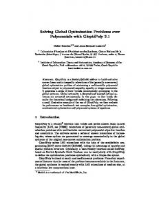
Figure 1: Six-hump camel back function. Consider the classical problem of minimizing globally the two-dimensional six-hump camel back function [4, Pb. 8.2.5] f (x1 , x2 ) = x21 (4 − 2.1x21 + x41 /3) + x1 x2 + x22 (−4 + 4x22 ). The function has six local minima, two of them being global minima, see figure 1.

2

To minimize this function we build the coefficient matrix   0

0 −4 0 0 0 0 0 0 0

 0 1  0  4  0 P = 0  −2.1 0   0 0 1/3

0 0 0 0 0 0 0

4 0 0 0 0 0 0

       

where each entry (i, j) in P contains the coefficient of the monomial xi1 xj2 in polynomial f (x1 , x2 ). We invoke GloptiPoly with the following Matlab script: >> P(1,3) = -4; P(1,5) = 4; P(2,2) = 1; >> P(3,1) = 4; P(5,1) = -2.1; P(7,1) = 1/3; >> output = gloptipoly(P); On our platform, a Sun Blade 100 workstation with 640 Mb of RAM running under SunOS 5.8, we obtain the following output: GloptiPoly 2.0 - Global Optimization over Polynomials with SeDuMi Number of variables = 2 Number of constraints = 0 Maximum polynomial degree = 6 Order of LMI relaxation = 3 Building LMI. Please wait.. Number of LMI decision variables = 27 Size of LMI constraints = 100 Sparsity of LMI constraints = 3.6667% of non-zero entries Norm of perturbation of criterion = 0 Numerical accuracy for SeDuMi = 1e-09 No feasibility radius Solving LMI problem with SeDuMi.. ... CPU time = 0.61 sec LMI criterion = -1.0316 Checking relaxed LMI vector with threshold = 1e-06 Relaxed vector reaches a criterion of -7.2166e-15 Relaxed vector is feasible Detecting global optimality (rank shift = 1).. Relative threshold for rank evaluation = 0.001 Moment matrix of order 1 has size 3 and rank 2 Moment matrix of order 2 has size 6 and rank 2 Rank condition ensures global optimality Extracting solutions.. Relative threshold for basis detection = 1e-06 Maximum relative error = 3.5659e-08 2 solutions extracted

3

The first field output.status in the output structure indicates that the global minimum was reached, the criterion at the optimum is equal to output.crit = -1.0316, and the two globally optimal solutions are returned in cell array output.sol: >> output output = status: 1 crit: -1.0316 sol: {[2x1 double] >> output.sol{:} ans = 0.0898 -0.7127 ans = -0.0898 0.7127

4

4.1

[2x1 double]}

GloptiPoly’s input: defining and solving an optimization problem Handling constraints. Basic syntax

Consider the concave optimization problem of finding the radius of the intersection of three ellipses [5]: max x21 + x22 s.t. 2x21 + 3x22 + 2x1 x2 ≤ 1 3x21 + 2x22 − 4x1 x2 ≤ 1 x21 + 6x22 − 4x1 x2 ≤ 1. In order to specify both the objective and the constraint to GloptiPoly, we first transform the problem into a minimization problem over non-negative constraints, i.e.  T    1 0 0 −1 1 min  x1   0 0 0   x2  x21 −1 0 0 x22   T   1 0 −3 1 1 s.t.  x1   0 −2 0   x2  ≥ 0 −2 0 0 x22 x21  T    1 1 0 −2 1  x1   0 4 0   x2  ≥ 0 x21 −3 0 0 x22    T  1 1 0 −6 1  x1   0 4 0   x2  ≥ 0. −1 0 0 x22 x21 4

Then we invoke GloptiPoly with a four-matrix input cell array: the first matrix corresponds to the criterion to be minimized, and the remaining matrices correspond to the non-negative constraints to be satisfied: >> >> >> >> >>

P{1} = [0 0 -1; P{2} = [1 0 -3; P{3} = [1 0 -2; P{4} = [1 0 -6; gloptipoly(P);

0 0 0 0

0 0; -1 0 0]; -2 0; -2 0 0]; 4 0; -3 0 0]; 4 0; -1 0 0];

When running GloptiPoly, we obtain an LMI criterion of −0.42701 which is a lower bound on the global minimum. Here it turns out that the computed bound is equal to the global optimum as shown in figure 2. 1.5

1

2x12+3x22+2x1x2=1 3x12+2x22−4x1x2=1 x12+6x22−4x1x2=1 x12+x22=0.4270

x2

0.5

0

−0.5

−1

−1.5 −2

−1.5

−1

−0.5

0 x1

0.5

1

1.5

2

Figure 2: Radius of the intersection of three ellipses.

More generally, when input argument P is a cell array of coefficient matrices, the instruction gloptipoly(P) solves the problem of minimizing the criterion whose polynomial coefficients are contained in matrix P{1}, subject to the constraints that the polynomials whose coefficients are contained in matrices P{2}, P{3}.. are all non-negative.

5

4.2

Handling constraints. General syntax

To handle directly maximization problems, non-positive inequality or equality constraints, a more explicit but somehow more involved syntax is required. Input argument P must be a cell array of structures with fields: P{i}.c - polynomial coefficient matrices; P{i}.t - identification string, either ’min’ - criterion to minimize, or ’max’ - criterion to maximize, or ’>=’ - non-negative inequality constraint, or ’> >> >> >> >> >> >>

P{1}.c = [0 -7 1; -12 0 0]; P{1}.t = ’min’; P{2}.c = [2 -1; 0 0; 0 0; 0 0; -2 0]; P{2}.t = ’==’; P{3}.c = [0; -1]; P{3}.t = ’ P.c(1,3,1,1,1,1,1,1,1,1) = 2; ... >> P.c(1,1,1,1,1,1,1,1,1,3) = 10; would create a 10-dimensional matrix P.c requiring 472392 bytes for storage. The equivalent instructions

7

>> >> >> >>

P.s = 3*ones(1,10); P.c = sparse(prod(P.s),1); P.c(sub2ind(P.s,3,1,1,1,1,1,1,1,1,1)) = 1; P.c(sub2ind(P.s,1,3,1,1,1,1,1,1,1,1)) = 2; ... >> P.c(sub2ind(P.s,1,1,1,1,1,1,1,1,1,3)) = 10; create a sparse matrix P.c requiring only 140 bytes for storage. Note however that the maximum index allowed by Matlab to refer to an element in a vector is 231 − 2 = 2147483646. As a result, if d denotes the maximum degree and n the number of variables in the optimization problem, then the current version of GloptiPoly cannot handle polynomials for which (d + 1)n > 231 . For example, GloptiPoly cannot handle quadratic polynomials with more than 19 variables.

4.4

DefiLin and DefiQuad: easy definition of linear and quadratic expressions

Linear and quadratic expressions arise frequently in optimization problems. In order to enter these expressions easily into GloptiPoly, we wrote two simple Matlab scripts called DefiLin and DefiQuad respectively. Refer to section 2 to download the Matlab source files defilin.m and defiquad.m. Given a matrix A and a vector b, the instruction P = defilin(A, b, type) allows to define a linear expression whose type is specified by the third input argument min - linear criterion Ax + b to minimize, or max - linear criterion Ax + b to maximize, or >= - inequality Ax + b ≥ 0, or =’. Output argument P is then a cell array of structures complying with the sparse syntax introduced in 4.3. There are as many structures in P as the number of rows in matrix A. Similarly, given a square matrix A, a vector b and a scalar c, the instruction P = defiquad(A, b, c, type) 8

allows to define a quadratic expression xT Ax + 2xT b + c. Arguments type and P have the same meaning as above. For example, consider the quadratic problem [4, Pb. 3.5]: min −2x1 + x2 − x3 s.t. xT AT Ax − 2bT Ax + bT b − 0.25(c − d)T (c − d) ≥ 0 x1 + x2 + x3 ≤ 4, 3x2 + x3 ≤ 6 0 ≤ x1 ≤ 2, 0 ≤ x2 , 0 ≤ x3 ≤ 3 where 

 0 0 1 A =  0 −1 0  −2 1 −1



 1.5 b =  −0.5  −5



 3 c= 0  −4



 0 d =  −1  . −6

To define this problem with DefiLin and DefiQuad we use the following Matlab script: >> >> >> >> >> >>

4.5

A = [0 0 1;0 -1 0;-2 1 -1]; b = [1.5;-0.5;-5]; c = [3;0;-4]; d = [0;-1;-6]; crit = defilin([-2 1 -1], [], ’min’); quad = defiquad(A’*A, -b’*A, b’*b-0.25*(c-d)’*(c-d)); lin = defilin([-1 -1 -1;0 -3 -1;eye(3);-1 0 0;0 0 -1], [4;6;0;0;0;2;3]); P = {crit{:}, quad, lin{:}};

DefiPoly: defining polynomial expressions symbolically

When multivariable expressions are not linear or quadratic, it may be lengthy to build polynomial coefficient matrices. We wrote a Matlab/Maple script called DefiPoly to define polynomial objective and constraints symbolically. It requires the Symbolic Math Toolbox version 2.1, which is the Matlab gateway to the kernel of Maple V [8]. See section 2 to retrieve the Matlab source file defipoly.m. The syntax of DefiPoly is as follows: P = defipoly(poly, indets) where both input arguments are character strings. The first input argument poly is a Maple-valid polynomial expression with an additional keyword, either min - criterion to minimize, or max - criterion to maximize, or >= - non-negative inequality, or > >> >> >> >> >>

P{1} P{2} P{3} P{4} P{5} P{6}

= = = = = =

defipoly(’min -12*x1-7*x2+x2^2’, ’x1,x2’); defipoly(’-2*x1^4+2-x2 == 0’, ’x1,x2’); defipoly(’0 output.sol{:}’ ans = -1.0000 -1.0000

-1.0000

1.0000

Another, classical integer programming problem is the Max-Cut problem. Given an undirected graph with weighted edges, it consists in finding a partition of the set of nodes into two parts so as to maximize the sum of the weights on the edges that are cut by the partition. If wij denotes the weight on the edge between nodes i and j, the Max-Cut problem can be formulated as P max 12 i> gloptipoly(defimaxcut(W), 3); to solve the third LMI relaxation, GloptiPoly returns the global optimum 12. Note that none of the LMI relaxation methods described in [1] could reach the global optimum.

5

GloptiPoly’s output: detecting global optimality and retrieving globally optimal solutions

GloptiPoly is designed to solve an LMI relaxation of a given order, so it can be invoked iteratively with increasing orders until the global optimum is reached, as shown in section 4.6. Asymptotic convergence of the optimal values of the relaxations to the global optimal 13

value of the original problem is ensured when the compact set of feasible solutions defined by polynomial inequalities satisfies a technical condition, see [6, 7]. In particular, this condition is satisfied if the feasible set is a polytope or when dealing with discrete problems. Moreover, if one knows that there exists a global minimizer with Euclidean norm less than M , then adding the quadratic constraint xT x ≤ M 2 in the definition of the feasible set will ensure that the required condition of convergence is satisfied. Starting with version 2.0, a module has been implemented into GloptiPoly to detect global optimality and extract optimal solutions automatically. The first output argument of GloptiPoly is made of the following fields: output.status - problem status; output.crit - LMI criterion; output.sol - globally optimal solutions. The following cases can be distinguished: output.status = -1 - the relaxed LMI problem is infeasible or could not be solved (see the description of output field sedumi.pinfo in section 6.1 for more information), in which case output.crit and output.sol are empty; output.status = 0 - it is not possible to detect global optimality at this relaxation order, in which case output.crit contains the optimum criterion of the relaxed LMI problem and output.sol is empty; output.status = +1 - the global optimum has been reached, output.crit is the globally optimal criterion, and globally optimal solutions are stored in cell array output.sol. See section 6.5 for more information on the way GloptiPoly detects global optimality and extracts globally optimal solutions. As an illustrative example, consider problem [4, Pb 2.2]: >> P = defipoly({[’min 42*x1+44*x2+45*x3+47*x4+47.5*x5’ ... ’-50*(x1^2+x2^2+x3^2+x4^2+x5^2)’],... ’20*x1+12*x2+11*x3+7*x4+4*x5= 0’, ’1-(x1-x2)^2 >= 0’,... ’1-(x2-3)^2 >= 0’}, ’x1,x2’); 22

The second LMI relaxation yields a criterion of −2 and moment matrices M12 and M22 of ranks 3 and 3 respectively, showing that the global optimum has been reached (since r = 1 here). GloptiPoly automatically extracts the 3 globally optimal solutions: >> [output, sedumi] = gloptipoly(P, 2); >> svd(sedumi.M{1})’ ans = 8.8379 0.1311 0.0299 >> svd(sedumi.M{2})’ ans = 64.7887 1.7467 0.3644 0.0000 0.0000 0.0000 >> output output = status: 1 crit: -2.0000 sol: {[2x1 double] [2x1 double] [2x1 double]} >> output.sol{:} ans = 1.0000 2.0000 ans = 2.0000 2.0000 ans = 2.0000 3.0000

6.6

Perturbing the criterion

When the global optimum is reached, another way to extract solutions can be to slightly perturb the criterion of the LMI. In order to do this, there is an additional field pars.pert - Perturbation vector of the criterion, default zero. The field can either by a positive scalar (all entries in SeDuMi dual vector y are equally perturbed in the criterion), or a vector (entries are perturbed individually). As example, consider the third LMI relaxation of the Max-Cut problem on the antiweb AW92 graph introduced in section 4.7. From the problem knowledge, we know that the global optimum of 12 has been reached, but GloptiPoly is not able to detect global optimality or extract optimal solutions. Due to problem symmetry, the LMI relaxed vector is almost zero:

23

>> [output, sedumi] = gloptipoly(P, 3); >> norm(sedumi.y(1:9)) ans = 1.4148e-10 In order to recover an optimal solution, we just perturb randomly each entry in the criterion: >> pars.pert = 1e-3 * randn(1, 9); >> [output, sedumi] = gloptipoly(P, 3, pars); >> output.sol{:}’ ans = Columns 1 through 7 -1.0000 -1.0000 1.0000 -1.0000 1.0000 Columns 8 through 9 1.0000 1.0000

6.7

-1.0000

-1.0000

Testing a vector

In order to test whether a given vector satisfies problem constraints (inequalities and equalities) and to evaluate the corresponding criterion, we developed a small Matlab script entitled TestPoly. The calling syntax is: testpoly(P, x) See section 2 to download the Matlab source file testpoly.m. Warning messages are displayed by TestPoly when constraints are not satisfied by the input vector. Some numerical tolerance can be specified as an optional input argument.

7 7.1

Performance Continuous optimization problems

We report in table 2 the performance of GloptiPoly on a series of benchmark non-convex continuous optimization examples. In all reported instances the global optimum was reached exactly by an LMI relaxation of small order, reported in the column entitled ’order’ relative to the minimal order of Shor’s relaxation, see section 4.6. CPU times are in seconds, all the computations were carried out with Matlab 6.1 and SeDuMi 1.05 with relative accuracy pars.eps = 1e-9 on a Sun Blade 100 workstation with 640 Mb of RAM running under SunOS 5.8. ’LMI vars’ is the dimension of SeDuMi dual vector y, whereas ’LMI size’ is the dimension of SeDuMi primal vector x, see section 6.1. Quadratic 24

problems 2.8, 2.9 and 2.11 in [4] involve more than 19 variables and could not be handled by the current version of GloptiPoly, see section 4.3. Except for problems 2.4 and 3.2, the computational load is moderate. problem [6, Ex. 1] [6, Ex. 2] [6, Ex. 3] [6, Ex. 5] [4, Pb. 2.2] [4, Pb. 2.3] [4, Pb. 2.4] [4, Pb. 2.5] [4, Pb. 2.6] [4, Pb. 2.7] [4, Pb. 2.10] [4, Pb. 3.2] [4, Pb. 3.3] [4, Pb. 3.4] [4, Pb. 3.5] [4, Pb. 4.2] [4, Pb. 4.3] [4, Pb. 4.4] [4, Pb. 4.5] [4, Pb. 4.6] [4, Pb. 4.7] [4, Pb. 4.8] [4, Pb. 4.9] [4, Pb. 4.10]

variables constraints degree LMI vars LMI size 2 0 4 14 36 2 0 4 14 36 2 0 6 152 2025 2 3 2 14 63 5 11 2 461 7987 6 13 2 209 1421 13 35 2 2379 17885 6 15 2 209 1519 10 31 2 1000 8107 10 25 2 1000 7381 10 11 2 1000 5632 8 22 2 3002 71775 5 16 2 125 1017 6 16 2 209 1568 3 8 2 164 4425 1 2 6 6 34 1 2 50 50 1926 1 2 5 6 34 1 2 4 4 17 2 2 6 27 172 1 2 6 6 34 1 2 4 4 17 2 5 4 14 73 2 6 4 44 697

CPU 0.41 0.42 3.66 0.71 31.8 5.40 2810 4.00 194 204 125 7062 3.15 4.32 7.09 0.52 2.69 0.72 0.45 1.16 0.57 0.44 0.86 1.45

order 0 0 +5 +1 +2 +1 +1 +1 +1 +1 +1 +2 +1 +1 +3 0 0 0 0 0 0 0 0 +2

Table 2: Continuous optimization problems. CPU times and LMI relaxation orders required to reach global optima.

7.2

Discrete optimization problems

We report in table 3 the performance of GloptiPoly on a series of small-size combinatorial optimization problems. In all reported instances the global optimum was reached exactly by an LMI relaxation of small order, with a moderate computational load. Note that the computational load can further be reduced with the help of SeDuMi’s accuracy parameter. For all the examples described here and in the previous section, we set pars.eps = 1e-9. For illustration, in the case of the Max-Cut problem on the 12-node graph in [1] (last row in table 3), when setting pars.eps = 1e-3 we obtain the global optimum with relative error 0.01% in 37.5 seconds of CPU time. In this case, it

25

means a reduction by half of the computational load without significant impact on the criterion. problem QP [4, Pb. 13.2.1.1] QP [4, Pb. 13.2.1.2] Max-Cut P1 [4, Pb. 11.3] Max-Cut P2 [4, Pb. 11.3] Max-Cut P3 [4, Pb. 11.3] Max-Cut P4 [4, Pb. 11.3] Max-Cut P5 [4, Pb. 11.3] Max-Cut P6 [4, Pb. 11.3] Max-Cut P7 [4, Pb. 11.3] Max-Cut P8 [4, Pb. 11.3] Max-Cut P9 [4, Pb. 11.3] Max-Cut cycle C5 [1] Max-Cut complete K5 [1] Max-Cut 5-node [1] Max-Cut antiweb AW92 [1] Max-Cut 10-node Petersen [1] Max-Cut 12-node [1]

vars 4 10 10 10 10 10 10 10 10 10 10 5 5 5 9 10 12

constr deg LMI vars LMI size 4 2 10 29 0 2 385 3136 0 2 385 3136 0 2 385 3136 0 2 385 3136 0 2 385 3136 0 2 385 3136 0 2 385 3136 0 2 385 3136 0 2 385 3136 0 2 385 3136 0 2 30 256 0 2 31 676 0 2 30 256 0 2 465 16900 0 2 385 3136 0 2 793 6241

CPU 0.33 10.5 7.34 9.40 8.25 8.38 12.1 8.37 10.0 9.16 11.3 0.35 0.75 0.47 63.3 7.21 73.2

order 0 +1 +1 +1 +1 +1 +1 +1 +1 +1 +1 +1 +2 +1 +2 +1 +1

Table 3: Discrete optimization problems. CPU times and LMI relaxation orders required to reach global optima.

8

Conclusion

Even though GloptiPoly is basically meant for small- and medium-size problems, the current limitation on the number of variables (see section 4.3) is somehow restrictive. For example, the current version of GloptiPoly is not able to handle quadratic problems with more than 19 variables, whereas it is known that SeDuMi running on a standard workstation can solve Shor’s relaxation of quadratic Max-Cut problems with several hundreds of variables. The limitation of GloptiPoly on the number of variables should be removed in the near future. GloptiPoly must be considered as a general-purpose software with a user-friendly interface to solve in a unified way a wide range of non-convex optimization problems. As such, it cannot be considered as a competitor to specialized codes for solving e.g. polynomial systems of equations or combinatorial optimization problems. It is well-known that problems involving polynomial bases with monomials of increasing powers are naturally badly conditioned. If lower and upper bounds on the optimization variables are available as problem data, it may be a good idea to scale all the intervals around one. Alternative bases such as Chebyshev polynomials may also prove useful. 26

Acknowledgments Many thanks to Claude-Pierre Jeannerod (INRIA Rhˆone-Alpes), Dimitri Peaucelle (LAASCNRS Toulouse), Jean-Baptiste Hiriart-Urruty (Universit´e Paul Sabatier Toulouse), Jos Sturm (Tilburg University) and Arnold Neumaier (Universit¨at Wien).

References [1] M. Anjos. New Convex Relaxations for the Maximum Cut and VLSI Layout Problems. PhD Thesis, Waterloo University, Ontario, Canada, 2001. See orion.math.uwaterloo.ca/∼hwolkowi [2] D. Bondyfalat, B. Mourrain, V. Y. Pan. Computation of a specified root of a polynomial system of equations using eigenvectors. Linear Algebra and its Applications, Vol. 319, pp. 193–209, 2000. [3] R. M. Corless, P. M. Gianni, B. M. Trager. A reordered Schur factorization method for zero-dimensional polynomial systems with multiple roots. Proceedings of the ACM International Symposium on Symbolic and Algebraic Computation, pp. 133–140, Maui, Hawaii, 1997. [4] C. A. Floudas, P. M. Pardalos, C. S. Adjiman, W. R. Esposito, Z. H. G¨ um¨ us, S. T. Harding, J. L. Klepeis, C. A. Meyer, C. A. Schweiger. Handbook of Test Problems in Local and Global Optimization. Kluwer Academic Publishers, Dordrecht, 1999. See titan.princeton.edu/TestProblems [5] D. Henrion, S. Tarbouriech, D. Arzelier. LMI Approximations for the Radius of the Intersection of Ellipsoids. Journal of Optimization Theory and Applications, Vol. 108, No. 1, pp. 1–28, 2001. [6] J. B. Lasserre. Global Optimization with Polynomials and the Problem of Moments. SIAM Journal on Optimization, Vol. 11, No. 3, pp. 796–817, 2001. [7] J. B. Lasserre. An Explicit Equivalent Positive Semidefinite Program for 0-1 Nonlinear Programs. SIAM Journal on Optimization, Vol. 12, No. 3, pp. 756–769, 2002. [8] Waterloo Maple Software Inc. Maple V release 5. 2001. See www.maplesoft.com [9] The MathWorks Inc. Matlab version 6.1. 2001. See www.mathworks.com [10] Y. Nesterov. Squared functional systems and optimization problems. Chapter 17, pp. 405–440 in H. Frenk, K. Roos, T. Terlaky (Editors). High performance optimization. Kluwer Academic Publishers, Dordrecht, 2000. [11] P. A. Parrilo. Structured Semidefinite Programs and Semialgebraic Geometry Methods in Robustness and Optimization. PhD Thesis, California Institute of Technology, Pasadena, California, 2000. See www.control.ethz.ch/∼parrilo 27

[12] J. F. Sturm. Using SeDuMi 1.02, a Matlab Toolbox for Optimization over Symmetric Cones. Optimization Methods and Software, Vol. 11-12, pp. 625–653, 1999. Version 1.05 available at fewcal.kub.nl/sturm/software/sedumi.html

28