May 9, 1989 - gence (A.I.) learning techniques is proposed. This algorithm, called GM-Learn, features a rudimen- tary learning mechanism which enables ...
GM-Learn : an iterative learning algorithm for CMOS gate matrix layout Sao-Jie Chen Yu Hen Hu
Indexing terms: Matrix algebra, Computer-aided design
Abstract: In the paper, an iterative CMOS gate matrix layout algorithm utilising artificial intelligence (A.I.) learning techniques is proposed. This algorithm, called GM-Learn, features a rudimentary learning mechanism which enables iterative improvements of the quality of a gate matrix layout. This is accomplished through the repetitive applications of a one-pass gate matrix layout algorithm, called GM-Plan, to realise a given circuit specification. The function of GM-Learn, is then to 'learn' to modify the heuristics used in GM-Plan based on the previous trials. Two AI learning paradigms, known as rote learning and learning by parameter adjustment, are employed. These learning techniques enable GM-Learn to modify its heuristic search parameters based on information obtained from previous iterations. Benchmark test results indicate that this novel algorithm is able to produce a high quality gate matrix layout in only a few iterations. The significance of this new method is that it may be applicable to other combinatorial VLSI physical design problems where heuristic guided search is required.
tions is displayed. In these simplified representations, it is implicitly assumed that the connections to the power sources (Vdd and GND) can easily be made once the gate placement and net routing are determined. 'dd
vss (i)
HVdd E metal
p-part net
diff.
n-part net VSS
a 1
1
Introduction
Gate matrix layout is a systematic CMOS layout methodology developed at Bell Laboratories [l]. Given a circuit schematic (Fig. l(i)) which consists of MOS transistors and interconnection wires (nets), a gate matrix layout maps MOS transistor gates (a and b) and input/ output nodes (c) into vertical columns using the polysilicon layer (Fig. l(ii)). Interconnection, power and ground wires are realised in metal wires running horizontally. A MOS transistor is formed when a horizontal diffusion layer wire (the drain and source of that transistor) overlaps the corresponding vertical polysilicon wire (the gate terminal of that transistor). Since the locations of MOS transistors are always on the intersections of (polysilicon gate) columns and (diffusion channel) rows, this layout style is thus called gate matrix layout. Often, symbolic representations are used to represent a gate matrix layout (e.g., Figs. l(iii) and l(iv)) so that only the essential information of gate placement and net connecPaper 72978 (C2, C4), received 14th February and in revised form 9th May 1989 Sao-Jie Chen is at the Department of electrical Engineering, National Taiwan University, Taipei, Taiwan, 10764, Republic of China Yu Hen Hu is at the Department of Electrical and Computer Engineering, University of Wisconsin - Madison, Madison, WI 53706, USA IEE PROCEEDINGS, Vol. 137, Pt. E, No. 4, JULY 1990
(ii)
b 2
c 3
gates slots
(iii) Fig. 1 N A N D circuit (i) Two-input NAND circuit (ii) Gate matrix layout (ii) Symbolic representation (iv)Symbolic layout
(iv)
The gate matrix layout features regular structure and relatively high gate density. These characteristics make it an increasingly popular design style for automated module generation in silicon compilers [2-51. However, the automatic generation of a high quality gate matrix layout is a difficult combinatorial optimisation problem. The objective of optimisation is to minimise the total number of rows (tracks) required in the gate matrix layout for a given circuit schematic. In designing a gate matrix layout, two basic tasks must be accomplished: the placement of all transistor gates and signal terminals to column slots and the routing of every net to horizontal tracks. It has been shown that this is an NP-complete problem [SI, of which an optimal solution is usually not easy to find. Instead, the application of heuristic approaches, though they may yield suboptimal solutions, seems to be more practical. Generally speaking, there are two distinct approaches to the gate matrix layout problem: the one-pass approach and the iterative approach. The one-pass 30 1
approach intends to find an acceptable solution is one single trial using the best possible heuristics, hence, its emphasis is on the efficiency of the algorithm. Examples of the one-pass approaches include : ‘Interval-graph’ method [7-lo], ‘net-ordering first’ method [ll, 123, ‘max-flow min-cut’ method [13, 141, ‘dynamic programming formulation’ [151,‘molecular physics modelling’ [2] and ‘AI planning’ [161 methods. On the other hand, the iterative approach attempts to improve a given solution by perturbing the existing one so as to minimise certain (heuristic) cost functions. Its emphasis is on the quality of the results. Examples of iterative methods include the ‘pairwise interchange’ method [5, 171 and ‘simulated annealing’ method [18]. In general, iterative methods are extremely time consuming. Our objective in this paper is to look for an iterative method, which is computationally more efficient than existing iterative methods and promises outputs of better quality than the one-pass algorithms. To achieve this goal, a novel iterative learning paradigm, called GMLearn, is proposed. A distinctive feature of GM-Learn is its incorporation of a one-pass algorithm, called GMPlan, into an iterative learning environment. This is accomplished by developing a learning scheme which utilises the one-pass GM-Plan to layout a given circuit for several consecutive runs (iterations). In each run, based on the previous outcome, the learning scheme modifies some of the parameters in the one-pass algorithm, with the hope that the quality of the present run will be improved. This learning paradigm closely mimics the problem solving strategy of human design engineers in that they can gradually improve the quality of the design by reworking on the same problem over and over again. In the domain of artificial intelligence research, the learning techniques adopted by the GM-Learn algorithm are known as a type of ‘rote learning’ and the ‘learning by parameter adjustment’ methods [191. These learning paradigms were originally utilised in the ‘checkers player’ program written by Samuel [20]. In applying these learning algorithms to our application domain-gate matrix layout, two questions have to be considered : what can be learned, and how to learn. In Samuel’s program, the subject to be learned is the estimated value of a heuristic cost function that guides the next move. Learning is accomplished from adjusting parameters (e.g. the weight of each factor) in this cost function so that it can predict the future outcomes more accurately and therefore achieve a better score. Weights of factors contributing to better outcomes will be reinforced. Otherwise, their values will be reduced. On analogy of the checkers player program, in this paper, the gate-placement heuristic cost function is the subject to be learned. Learning is accomplished by combining estimates obtained from the previous solution with current estimates. The weights of combinations depend on the quality (number of tracks used) of the previous solution. Although this is a rather rudimentary learning technique, significant reductions in track usage in gate matrix layout have been observed from simulation examples. It should be noted here that similar iterativeimprovement methods have also been used in the task of global routing for IC components in the past [21, 223. These methods repeatedly improve their previous solutions with a technique called ‘rip-up routing’. This technique re-routes one net at a time according to a newly calculated and, hopefully, a better estimated cost function, named ‘penalty’ [21] or ‘cell boundary demand’ [22]. To the best of our knowledge, no similar iterative 302
method has been proposed for improving the gate matrix layout. 2
Reviews of the one-pass algorithm: GM-Plan
GM-Plan is an AI planning-based one-pass gate matrix layout algorithm developed by the authors recently [161. The gate matrix layout problem is formulated, in GMPlan, as a planning problem in which the overall goal of layout is decomposed into a set of subgoals (subproblems). Each subgoal corresponds to the placement of a gate and the assignment of tracks to the nets connecting to that gate. Since subgoals interact with each other and compete for resources (uses of tracks), unnecessary tracks may be added due to inappropriate management of subgoal interactions. In GM-Plan, this problem is resolved by employing two meta-planning control policies, called the graceful retreat (GR) policy and the least impact (LI) policy. The GR policy gives high priorities to subgoals which are less flexible, or more difficult, to accomplish. The LI policy directs the program to look for, among a set of potential solutions, the one that interferes the least with solutions of other subgoals. In GM-Plan, each subgoal is accomplished in four steps : ( a )Choose a gate to be placed next. ( b ) Select a slot to place that gate. (c) Choose a set of nets to be routed to that gate. (d) Select tracks to route the set of chosen nets. The second step is the most critical one as it imposes a gate ordering constraint which has profound effects on the remaining solutions. In GM-Plan, this step is accomplished under the control of the LI policy. Specifically, a heuristic cost function is evaluated for each potential slot. The lower the cost, the less resources that will be required (therefore, the less impacts that there will be on the remaining solutions). Unfortunately, because of the interaction among subgoals, the cost function can not be evaluated accurately without exhaustive enumeration. Hence, certain factors of the cost function must be estimated using heuristics. Naturally, the more accurately the cost function is evaluated, the better the gate matrix layout would be. Suppose that results of previous runs are available, it might be possible to deduce more accurate estimates in the current run. This is exactly the approach taken by GM-Learn. 3
Improving gate matrix layout quality with learning
Learning denotes changes in the system that are adaptive in the sense that they enable the systems to do the same task or tasks drawn from the same population more efficiently and more eflectively the next time. Herb Simon [23]
The main learning method used in this paper can be regarded as a technique of ‘learning by parameter adjustment’ [19]. The basic idea of this approach is to run the one-pass GM-Plan algorithm on the same given circuit netlist several times. With each run, hopefully, the algorithm will be able to improve its performance using results from the previous run. This is analogous to human designers who improve their problem solving skills (in this case, the gate matrix layout) by solving IEE PROCEEDINGS, VoI. 137, P t . E, No. 4, J U L Y 1990
(practising) the same problem repeatedly. The bottom line is that the experience obtained from early trials can be utilised to improve the solution quality of the same problem. In some sense, this is a process of learning by practising. 3.1 Applications of A. 1. learning techniques Two learning methods are used in GM-Learn. One of the methods is the application of an AI ‘learning by parameter adjustment’ method developed in Samuel’s checkers player program (cf. Chap. XIV, Sec. D5a in Reference 24). An analogy is drawn between the tasks of checkers playing and of the gate matrix layout: both of them involve a combinatorial search through the solution space where a ‘good’ heuristic move (solution step) relies on the accurate prediction (look ahead) of consequences of the current move. In the checkers player program, a linear heuristic cost function was used to evaluate the potential benefit of making a specific move. While in the one-pass GM-Plan gate matrix layout algorithm, a similar linear heuristic cost function (to be described later) is used to determine which slot should be used to place the current gate. Hence, it is natural to use the same learning technique to help improve the estimate of the cost function. Another learning method used in Samuel’s checkers player program (cf. Chap. XIV, Section B2 in Reference 24), and in GM-Learn also, is called ‘rote learning’. Rote learning is a mechanical learning paradigm in which learning means to memorise a large amount of raw information without further processing [24]. In Samuel’s checkers player program, the cost of a move is retrieved from a data base rather than re-evaluation. Similarly, in gate matrix layout, results of the previous solution are retained to be used by the learning algorithm. To apply these two AI learning paradigms, a two-step approach has been taken in GM-Learn: (i) identify the set of parameters as the subject to be learned, and this should answer the question, ‘what can be learned? (ii) develop a set of learning rules to adjust the identified set of parameters in order to produce desired outputs, and this responds to the question, ‘how to learn?
3.2 What can be learned? The heuristic cost function in the one-pass algorithm GM-Plan for slot selection is the subject to be learned in GM-Learn. This cost is an estimate of the total wire lengths required when the current gate is placed in a particular slot. According to the least impact policy, the slot with the lowest cost is favoured as it minimises the impacts on the routing of nets corresponding to gates which have not yet been placed. This cost function, denoted by f, can be further decomposed into four factors :
f = g l (connection cost of fixed nets)
+ h l (expansion cost of fixed nets) + h2 (connection cost of floating nets) + h3 (expansion cost of floating nets). Each of these factors will be described in detail below. In GM-Plan, a net will be committed to a track only if most of the gates connecting to this net have been placed. Once a net is assigned to a track, it is called a fixed net. IEE PROCEEDINGS, Vol. 137, Pt. E, N o . 4, J U L Y 1990
Otherwise, the routing of the net will be postponed until later steps of design. Such a net is called a floating net. When a gate is placed into a particular slot, two situations may occur: For those nets which connect to the current gate, a connection is made. The increase in net lengths due to the connection of nets to the newly placed gate is called the connection cost. The other situation is that the placement of a new gate may cause other existing nets to be stretched. The amount of stretching (expansion) is called the expansion cost. Combining these two types of nets with these two situations, we have the four factors contributing to the cost functionf: A possible scenario of the four cases is depicted in Fig. 2. (a) g l is called the fixed net connection cost. In Fig. 2, n l and n2 are fixed nets that have been connected to other gates. Since they all connect to the current gate 9, each of them has a connection cost. To estimate gl, if a fixed net has already been connected to two sides of 9, only one unit will be assigned (e.g. nl). If a net connects to only one side of g, the actual distance is used as its cost (e.g. cost for n2 is 2). Since all fixed nets are already in place, the cost of g l (in this example, it is 3) can be estimated fairly accurately.
Heuristic cost functions net connection = floating net connection
Fig. 2
x = fixed
(b) hl is called the fixed net expansion cost. It estimates the possible expansion lengths of fixed nets that do not connect to the gate 9. Since its value depends on the future placement of remaining gates, in GM-Plan, it is simply assigned with a unity value for each of these fixed nets. Refer to Fig. 2, in that example, the example of h l is 2. (c) h2 is called the floating net expansion cost. Again, its value cannot be enumerated. In GM-Plan, we only count the number of floating nets and multiply this count by 0.5. Thus, in Fig. 2, h2 = 0.5 * 2 = 1. (d) h3 is called the floating net connection cost. Its definition is similar to that of h l above. The same method as in the case of h2 is applied to estimate its value. Again, refer to Fig. 2, the estimate of h3 is h3 = 0.5 * 2 = 1. From the above discussions, the cost off is thus equal to 7 (= 3 + 2 1 1). The values of the last three factors (namely, hl, h2, and h3 in the cost functionf) need to be estimated heuristically as they depend on the outcome of future layout steps. If the current solution does not deviate dramatically from the previous one, then the values of these cost functions evaluated based on the previous solution may serve as better estimates than those obtained by using only heuristics. In other words, h l , h2, and h3 are to be learned.
+ +
303
3.3 How to learn? Once a set of parameters (in the cost functionf) is identified as the subject to be learned, the next question to ask, then, should be
ezoid rule usually gives better results than the other two rules. 3.4 Other improvement heuristics With the existence of a previous solution, some of the design heuristics used in GM-Plan may be relaxed in GM-Learn to improve the layout. One of these heuristics is devised for the slot assignment process after a candidate gate is selected. To keep the search process efficient, in GM-Plan, the cost function of those slots whose neighbouring gates have no direct connection (via one or more nets) with the to-be-placed gate will not be evaluated. Furthermore, using the seed gate’ as a ‘continental divide’, only one side of the seed gate which has more potential slots will be searched. In GM-Learn, the search process will be extended to all the neighbouring gates of the placed gate (including both sides of the seed gate) whenever the previous outcome suggests so. Another type of heuristic which may be improved with an existing solution is the heuristic of assigning (routing) nets to tracks. At the routing stage of GM-Plan, we avoid using the track reserved by a fixed net, which is not completely connected to its constituent gates. This conservative approach is due to the lack of a complete layout information. In GM-Learn, this (heuristic) restriction can also be relaxed taking advantage of the availability of a previous solution.
How do we adjust these parameters so as to learn to improve the overall gate matrix layout quality ?
Since the relation between the parameters and the output quality is highly non-linear, it is unlikely that an analytical model can be derived to describe the behavior of a gate matrix layout algorithm in terms of those identified parameters (e.g. h l , h2, and h3). Two extreme cases can be identified. One is to ignore completely the existence of a previous solution of the same problem, and to use only the original heuristics as if that solution does not exist. The other is to directly substitute these parameter values with those calculated from the previous solution; this may ignore the potential difference between the current solution and the previous solution. A compromise between these two extreme choices would be to take a weighted average of these two estimates. In developing GM-Learn, these three types of heuristic rules for adjusting parameters are all implemented and tested. These rules are called’ forward Euler, backward Euler, and trapezoid rules. (i) Forward Euler rule: This is the heuristic which ignores completely the existence of previous solutions, and uses only the ‘guessed’ values of the three components, h l , h2, and h3, in the heuristic cost functionf: (ii) Backward Euler rule: This is the other extreme that uses solely the calculated values of h l , h2 and h3 from the previous solution as the estimates of the current run, (iii) Trapezoid rule : This heuristic takes a weighted average of the guessed (in the current run) and the calculated (from the previous output) values of h l , h2, and h3.
4
Algorithm formulation and complexity analysis
The main procedure of GM-Learn is outlined below, where in line 2, ‘c’ is the iteration count. In line 3, oldNO and oldGO (ONO and oGO in GM-Plan and GMLearn) are the status tables used to store the information of the previous solution while newNO and newGO (nNO and nGO in GM-Plan and GM-Learn) are used to store the information generated by the current iteration.
With the many simulation results we have tried, the trap~
Algorithm Main: 1 { GM-Plan (NG, GN, oldNO, oldGO); 2 for (i = 1 to c) 3 { GM-Learn (NG, GN, oldNO, oldGO, newNO, newGO); 4 oldNO = newNO; 5 oldGO = newGO; 6 1 7 choose the best solution as output. 8 1 Algorithm GM-Plan (NG, GN, ONO, oGO):
l
/*First planning iteration */ /*Learning iterations */ /*Update oldNO, oldGO with newNO and newGO */
/*Prepare net-gate tables */ /*Place the first seed gate and route its nets */ /*Form the NearestNeighboring Gate group */ /*Form Current Gate-Set */
Prepare-Table (NG, GN); Unique-pl&route ( ); Form-NNG (); CRGS = NNG; Layout 0 { While (CRGS != NULL) repeat { Place-gate ()
/*Gate Placement procedure using planning techniques */
{ select (g, CRGS) with GR policy; plan-place (g, slot, ONO, oGO) with L1 policy; update (ONO, oGO);
I A seed gate is the gate that connects to a maximum number of nets.
In GM-Plan, it is selected as the first gate to be placed. Then, the other We borrow these names from the calculus literature where these rules are applied in doing numerical integration. 304
gates will be placed based on their connectivity with respect to this gate. Hence,it is called the seed gate. IEE PROCEEDINGS, Vol. 137, Pt. E, No. 4, JULY 1990
1
/*Net Routing procedure */
Route-net (N(g)) if (end of NNG) deferred-route (N(sg)); PLGS = PLGS U {g}; CRGS = {CRGS U G(N(g))}\PLGS;
/*Update PLaced Gate Set/ /*Update Current Gate Set */ /*end of While loop */
1
1
/*Check for unrouted nets
WrapupRoute (all-nets).
*/
1
Algorithm GM-Learn (NG, GN, ONO, oGO, nNO, nGO): /*Place the first seed gate and route its nets */ /*Form the NearestNeighboring Gate group */ /*Form Current Gate-Set */
Unique-pl&route (); Form-NNG (); CRGS = NNG; Layout ( ) { While (CRGS ! = NULL) repeat { Place-gate ( )
/*Gate Placement procedure using learning techniques */
{ select (g, CRGS) with GR policy; learn-place (g, slot, ONO, oGO, n N 0 , nGO) with Learning & LI policy; update (ONO, oGO, nNO, nGO);
1
/*New Routing procedure
Route-net (N(g)) if (end of NNG) deferred-route (N(sg)); PLGS = PLGS U (8); CRGS = {CRGS U G(N(g))}\PLGS;
1
/*Update PLaced Gate Set */ /*Update Current Gate Set */ /*end of While loop */
1
/*Check for unrouted nets */
WrapupRoute (all-nets). In the above formulation, the original one-pass algorithm GM-Plan is applied initially, since there are no ‘previous’ results available at that time. The main difference between GM-Plan and GM-Learn is in the gate placement step where plan-place() is used in GM-Plan, and learn-place() in GM-Learn. The procedure ‘plan-place’ uses only guessed values to calculate the cost functionf and stores its layout results in the ONO and oGO tables The parameter adjustment learning algorithm is implemented in the procedure ‘learn-place’ using ‘learned’ values stored in the ONO and oGO tables. The improved slot-assignment heuristic (discussed in Section 3.4) is encoded in the procedure ‘learn-place’. The modified track-assignment (net routing) heuristic of Section 3.4 is implemented in the procedure ‘Route-net’ of GM-Learn. As far as computational complexity is concerned, since GM-Learn essentially consists of multiple runs of a slightly modified version of the one-pass GM-Plan algorithm, the total operation count may be estimated as a product of the total number of iterations c and the operation count of the GM-Plan algorithm. It has been shown that the total number of computations required in GM-Plan is O(n2m), where n is the number of gates and m is the total number of nets to be routed [16]. Thus, the computation complexity of the GM-Learn algorithm should be of O(cn2m). It is important to note that in actual implementation, to be efficient, the iteration count c should be kept small. 5
GM-Learn is able to reduce the total number of tracks from six to four (Fig. 3C), which is the optimal solution. Plots of Figs. 3B and 3C are given in Figs. 3D and 3E, respectively. circuit x 7
7
48 5678 5678
nets-7 gates-8 a Fig. 3A Net-gate table
IEE PROCEEDINGS. Vol. 137, Pt. E , No. 4, JULY 1990
of x7
23415678
xx xxxxxx
total tracks=6
b Fig. 38
Result afterfirst pass
15263784
Implementation results
5.1 Examples First, a simple circuit netlist ‘x7’ consisting of eight transistors (gates) and seven nets is given in Fig. 3A. After the first iteration, that is, the one-pass application of the GM-Plan algorithm, it was found that six tracks are used as depicted in Fig. 3B. However, after the 3rd iteration,
*/
x-x-x x-x-x x-x-x-
i=0 i- 1 i- 2 i 3
track track track track i = 4 track i 5 track
x x
-x C
Fig. 3C
-
-
=6
6 1 4 =4 =4
=4
Result after 6 passes
305
Fig. 3D
.>
select place.
Fig. 3E 306
Plot of result afterfirst pass
leave
oad L i b r a n da2.crl Ok1
Plot ofresult after 6 passes I E E PROCEEDINGS, Vol. 137, Pt. E, No. 4, JULY 1990
As another example, a circuit ‘xo’containing 48 transistors (gates) and 40 nets is shown in Fig. 4A. At the end of the first iteration, 15 tracks are required (Figs. 4B and 4D); this is equal to the solution given in the literature [25]. However, after the 3rd and the 6th iterations, the track number is reduced to 13 Figs. 4C and 4E). Circuit x 0 Gate
Net Gate
Net 1 2 3 4 5 6 7 8 9 10 11 12 13 14 15 16 17 18 19 20
-
1 2 3 4 7 8 29 30 31 32 33 23 24 1 4 7 11 12 8 13 20 6 19 28 45 47 48 1 3 11 5 6 35 37 38 18 23 26 2 4 5 9 10 6 29 38 46 47 48 2 3 9 12 14 22
21 22 23 24 25 26 27 28 29 30 31 32 33 34 35 36 37 38 39
40
25 27 28 43 44 12 15 32 19 20 21 22 23 18 44 45 12 16 42 26 27 28 18 24 25 8 28 30 10 21 38 18 33 36 8 38 40 18 34 35 39 40 41 42 43 33 34 10 31 48 18 43 46 10 17 41 6 39 48 36 37 38 nets = 40 gates = 48
Fig. 4A
Net-Gate table of x0
4311 434444444133333322222212 23111 13221 1 817092431902763548364785543679916582265171002483
It is interesting to note that the reduction in track number is not monotonic. In other words, the GM-Learn has the potential to skip a local minimum in search of the nearby global minimum at the risk of finding a worse solution during the problem solving process. If the global optimal solution is too far away, then it is possible that GM-Learn will yield solutions inferior to the first pass solution. In this case, the initial solution will be taken as the best one obtained. In fact, in our testing of several benchmark examples, this case did occur in a circuit ‘w3’ as discussed below.
5.2 Benchmark test results Two sets of benchmark circuits have been used to test the effectiveness of the proposed GM-Learn algorithm. The first set of 16 circuits are collected from the published literature as indicated in Table 1. The ‘lower bound’ column in the Table equals the maximum number of nets connected to a gate in each circuit. If the track number used in the layout is equal to this lower bound, an optimal solution is obtained. However, the optimal solution may require more tracks than the lower bound. In the case of simple circuits, the optimal track number can be found by an exhaustive search. If the track number listed in the table is followed by an asterisk, then it is an optimal solution. The column ‘known solution’ denotes the best solution found in the literature. The column under the title ‘planning solution’ gives the required track number after the first iteration. The ‘learning solution’ column gives the track number after six iterations. If after the last iteration, no solution is better than the first planning solution, the track number will be enclosed in parentheses as shown in circuits ‘w3’ and ‘wsn’. The last column listed the CPU time taken on a VAX 11/750 minicomputer. At current time, since the program is not fully polished, it may take too much memory space and could not be run on a VAX 11/750 for some large circuits, such as circuits ‘w3’ and ‘w4‘. The results for these circuits are obtained by running the algorithm on a Sequent Symmetry S81 computer which has a larger memory and faster processors. In Table 1, it is observed that out of the 16 test circuits, GM-Learn successfully improved the results obtained from the one-pass GM-Plan in eight cases (i.e. ‘v~OOO’, ‘v4050’, ‘vWo’, ‘v447o’, ‘w4, ‘wli’ and ‘xo’), produced equally good (and optimal) results in six cases (i.e. ‘vl’, ‘vwl’ ‘vw~’,‘wl’, ‘w2’ and ‘wsn’), and yielded worse results in two cases only (i.e. ‘w3’ and ‘wsn’). Compared with the twelve known results (of which only nine were Table 1 : Gate matrix layout results w i t h GM-Learn
name of lower known planning learning CPU time test circuits bound solution solution solution vax 750s and sources Or#) Or#) Or#)
total tracks = 13 i = 0 track = 15 i = 1 track = 15 i = 2 track = 13 i = 3 track = 17 i = 4 track = 14 i = 5 track = 13 Fig. 4C Result after 6 passes of GM-Learn
IEE PROCEEDINGS, Vol. 137, Pt. E, No. 4, JULY I990
v4000 [26] v4050 [26] v4090 [26] v4470 [26] VCI [2] VI[18] vwl [8] vw2 [9] w l [SI w2 [27] w3 [27] w4 [27] wan [27] wli [lo] wsn [28] x0 [25]
5 5 9 5 9
3 4 3 4 14 11 18 6 4 4 6
9’ 3* 4* 5* 4* 14* 23 36 6* 4* 8* 15
7 6 11 14 10 3. 42 5* 4* 14* 21 46 6* 6 8* 15
6 5* 10* 11 9* 3* 4*
5’ 4. 14* (23-25) 34 6’ 4* (10) 13
16.7 13.1 43.1 73.2 36.1 3.2 3.1 4.9 12.8 66.8 N/A N/A 4.1 6.4 23.6 102.0
307
Fig. 4D
Plot of result aftterfirst pass
Fig. 4E
Plot of GM-Learnresult after 6 passes
308
-
IEE PROCEEDINGS, Vol. 137, Pt. E, No. 4, JULY 1990
~~
optimal solutions), GM-Learn yielded better results in two of the three non-optimal (non-starred) cases (i.e. ‘w4‘ and ‘xo’), and the first one-pass GM-Plan also outperformed the known result in the last case (‘w3’). If we record all the results obtained while running GM-Learn and take the best one (either generated by GM-Learn or by GM-Plan) as the final results, it may be claimed that GM-Learn performs better or equally well compared with existing methods in these testing cases.
5.3 Discussion The second set of sample circuits, taken from [lS], can be used to judge whether a gate matrix layout algorithm is a ‘greedy algorithm’. A greedy algorithm is the steepest descent type algorithm which always makes a move that yields a maximum reduction in the cost function of the current step. Thus, a greedy algorithm, though usually is more computationally efficient, may get stuck at a local minimum. From Table 2, it is observed that the one-pass GM-Plan algorithm is closer to a ‘greedy’algorithm as it yielded suboptimal solutions for three out of the nine test circuits. However, with GM-Learn, all results are optimal. Moreover, if convergence occurs, as most test cases do, it occurs within very few iterations. Hence we are optimistic that this algorithm could be a practical candidate for larger-scale gate matrix layout problems. This compares favourably with other iteration methods, such as the pairwise interchange method [17], which takes (O(n*2(”-”)) time to achieve an optimal solution; or the ‘simulated annealing’ method [18], which also takes extremely long computation time, even using a reasonable cooling schedule. Table 2: Special gate matrix layout results with G M Learn
name of circuits
lower bound
known solution Or#)
planning solution Or#)
learning solution (tr # )
CPU time vax 750 s
xl x2 x3 x4 x5 x6 x7 x8 x9
2 2 2 2 2 2 3 3 3
5* 6* 7* 2* 2* 2* 4* 4* 4*
5* 6* 7* 2* 2* 2* 6 10 18
5’ 6* 7* 2* 2* 2* 4* 4* 4*
6.7 13.2 24.0 3.1 8.3 24.4 4.9 15.5 58.6
6
Conclusion and future research directions
In this paper, learning paradigms developed in the artificial intelligence research have been applied to derive an iterative learning gate matrix layout algorithm - GMLearn. The two important questions in deriving a learning algorithm, ‘what can be learned’ and ‘how to learn’, were answered in the context of GM-Learn with the use of a one-pass algorithm GM-Plan. Benchmark examples showed that GM-Learn is able to generate optimal solutions in relatively few iterations in many cases. Besides the achievements presented in this paper, many open questions still remain to be studied, some of which are listed below: (a) how to further improve the efficiency of the GMLearn algorithm (b) how to apply the iterative learning paradigm to other one-pass layout algorithms, and perhaps to general CAD algorithms where heuristic search is required (c) how to apply more sophisticated learning paraIEE PROCEEDINGS, Vol. 137, Pt. E, No. 4 , J U L Y 1990
digms developed in the field of A.I. to the gate matrix layout problem, or to the general CAD problems. To find the answers to the above questions, further research is certainly needed. However, the payoff in the long run, we believe, will justify such efforts. 7
References
1 LOPEZ, A.D., and LAW, H-F.S.: ‘A dense gate matrix layout method for MOS VLSI’, IEEE Trans., 1980, ED-27, (8), pp. 16711675 2 CHANG, Y.C., CHANG, S.C., and HSU, L.H.: ‘Automated layout generation using gate matrix approach’, Proc. 24th Design Automation CO?$, 1987, pp. 552-558 3 CHEN, J.S-J., and CHEN, D.Y.: ‘A Design Rule Independent Cell Compiler’, Proc. 24th Design Automation Cont. 1987, pp. 466471 4 LIN, Y-L.S., and GAJSKI, D.D.: ‘LES: A layout expert system’, Proc. 24th Design Automation Cont. 1987, pp. 672478 5 YU, M.L., and KUBITZ, W.J.: ‘A VLSI cell synthesizer with structural constraint considerations’, Proc. Int. Con5 Computer-Aided Design, 1985, pp. 58-60 6 KASHIWABARA, T., and FUJISAWA, T.: ‘A NP-complete problem on interval graph’, Proc. Int. Symposium on Circuits and Systems, 1979, pp. 82-83 7 OHTSUKI, T., MORI, H., KUH, E.S., and FUJISAWA, T.: ‘Onedimensional logic gate assignment and interval graph’, IEEE Trans., 1979, CAS-26, (9), pp. 67-84 8 WING, 0.: ‘Automated gate matrix layout’, Proc. Int. Symposium on Circuits and Systems, 1982, pp. 681-685 9 WING, O., HUANG, S., and WANG, R.: ‘Gate matrix layout’, IEEE Trans., 1985, CAD-4, (3), pp. 220-231 10 LI, J.T.: ‘Algorithms for gate matrix layout’, Proc. Int. Symposium on Circuits and Systems, 1983, pp. 1013-1016 11 ASANO, T., and TANAKA, K.: ‘A gate placement algorithm for onedimensional arrays’, J. of Information Processing, 1978, 1, (l), pp. 47-52 ‘Improved gate matrix layout’, Proc. 12 HUANG, S., and WING, 0.: Int. Con/. Computer-Aided Design, 1986, pp. 320-323 13 CHENG, C.K.: ‘Decomposition algorithms for linear placement and application to VLSI design’, Proc. Int. Symposium on Circuits and Systems, 1985, pp. 1047-1050 14 HWANG, D.K., FUCHS, W.K., and KANG, S.M.: ‘An efficient approach to gate matrix layout’, IEEE Trans., 1987, CAD-6, (9,pp. 802-809 15 DEO, N., KRISNAMOORTHY, M.S., and LANGSTON, M.A.: ‘Exact and approximate solutions for the gate matrix layout problem’, IEEE Trans., 1987, CAD-6,(l),pp. 79-84 16 HU, Y.H., and CHEN, S.J.: ‘GM-Plan: A gate matrix layout algorithm based on AI planning techniques’, Proc. Int. Symposium on Circuits and Systems, 1989, pp. 1867-1870 17 YOSHIZAWA, H., KAWANISHI, H., and KANI, K.: ‘A heuristic procedure for ordering MOS arrays’, Proc. 12th Design Automation Conf, 1975, pp. 384393 18 LEONG, H.W.: ‘A new algorithm for gate matrix layout’, Proc. Int. ConJ Computer-Aided Design, 1986, pp. 316-319 19 RICH, E.: ‘Artificial Intelligence’ (McGraw-Hill, Inc., New York, 1983) 20 SAMUEL, A.L.: ‘Some studies in machine learning with the game of checkers’, IBM J. Res. Develop., 3, 1959, pp. 210-220 21 LINSKER, R.: ‘An iterative-improvement penalty-functiondriven wire routing system’, IBM J. Res. Develop., 1984, 28, (5), pp. 613424 22 NAIR, R.: ‘A simple yet effective technique for global wiring’, IEEE Trans., 1987, CAD-6, pp. 165-172 23 SIMON, H.A.: ‘Why should machines learn?’, in MICHALSKI, R.S., CARBONELL, J.G. and MITCHELL, T.M. (Eds.): ‘Maching Learning: An artificial intelligence approach’ (Tioga, Palo Alto, Calif., 1983) 24 BARR, A., and FEIGENBAUM, E.A. (Eds.): ‘The handbook of artificial intelligence, Volume 111’ (William Kaufman Inc., New York, 1982), chap. XIV 25 NAKATANI, K., FUJII, T., KIKUNO, T., and YOSHIDA, N.: ‘A heuristic algorithm for gate matrix layout’. Proc. ICCAD, 1986, pp. 324327 26 HEINBUCH, D.V. : ‘CMOS Cell Library’ (Addison-Wesley, Reading, MA, 1988) 27 HUANG, S., and WING, 0.:‘Improved gate matrix layout’, IEEE Trans., 1989, CAD-8, (8), pp. 875889 28 WING, 0.: ‘Interval graph based circuit layout’. Proc. ICCAD, 1983, pp. 84-85 309