GMM improves the reject option in hierarchical classification for fish recognition Phoenix X. Huang School of Informatics University of Edinburgh 10 Crichton street, Edinburgh
Bastiaan J. Boom School of Informatics University of Edinburgh 10 Crichton street, Edinburgh
Robert B. Fisher School of Informatics University of Edinburgh 10 Crichton street, Edinburgh
[email protected]
[email protected]
[email protected]
Abstract A reject option in classification is useful to filter less confident decisions of known classes or to detect and remove untrained classes. This paper presents a novel rejection system in a hierarchical classification method for fish species recognition. Since hierarchical methods accumulate errors along the decision path, the rejection system provides an alternative channel to discover misclassified samples at the leaves of the classification hierarchy. This is also applied to probe test samples from new classes. We apply a Gaussian Mixture Model (GMM) to evaluate the posterior probability of testing samples. 2626 dimensions of features, e.g. color and shape and texture properties, from different parts of the fish are computed and normalized. We use forward sequential feature selection (FSFS), which utilizes SVM as a classifier, to select a subset of effective features that distinguishes samples of a given class from others. After learning the mixture models, the reject function is integrated with a Balance-Guaranteed Optimized Tree (BGOT) hierarchical method. We compare three rejection methods. The experimental results demonstrate a reduction in the accumulated errors from hierarchical classification and an improvement in discovering unknown classes.
1. Introduction Computer vision and pattern recognition techniques can help biologists observe marine ecosystems. These techniques help detect significant events or objects and filter out most worthless content from mass video databases. Vision techniques, when integrated with marine knowledge, can analyse underwater objects and compose high level interpretation, like fish counting, fish species distribution variation, fish behaviour pattern, from a Tera-scale video database. The marine scientists benefit from the computingassisted analysis of underwater videos, e.g. fish detection and species recognition, for long-term observation [20]. Live fish recognition in the open sea promotes commercial
and environmental applications like fish farming and meteorological monitoring [12]. Traditionally, marine biologists have employed many tools to examine the appearance and quantities of fish. For example, they cast nets to catch and recognize fish in the ocean. They also dive to observe underwater, using photography [3]. Moreover, they combine net casting with acoustic (sonar) [2]. Nowadays, much more convenient tools are employed, such as hand-held video filming devices [11]. Embedded video cameras are also used to record underwater animals (including insects, fish, etc.), and observe fish presence and habits at different times [15]. This equipment has produced large amounts of data and it requires informatics technology like computer vision and pattern recognition to analyse and query abundant videos. Statistics about specific oceanic fish species distribution, besides an aggregate count of aquatic animals, can assist biologists resolving issues ranging from food availability to predator-prey relationships [10]. However, the recognition task is fundamentally challenging because fish can move freely and illumination levels change frequently in such environments [19, 17]. The fish recognition task is an application of multi-class classification. A common multi-class classifier could be considered as a flat classifier because it classifies all classes using the same features at the same time [4]. A critical drawback is that it does not consider certain similarities among classes. These classes can be better separated by specifically selected features. One solution is to integrate domain knowledge and construct a tree to organize these classes hierarchically [6], called hierarchical classification. This method has significant advantages by grouping similar classes into certain subsets and selecting specific subsets of features to distinguish them at a later stage [9]. Hierarchical structures are popular in document and image categorization. Mathis [13] organizes documents hierarchically by making use of the correlations between topical subjects. Deng et.al. [7] introduced a new dataset called ImageNet where a large scale hierarchical ontology of images are constructed based on the WordNet knowledge. One problem
with these hierarchical classification methods is the error accumulation. Each level of the hierarchical tree has some classification errors. In fish recognition, especially when our database is extremely imbalanced, misclassified samples are passed into deeper layers and reduce the average accuracy of the final recognition performance. Another issue for a multi-class classifier (not only for hierarchical classification) is that it classifies every test sample into one of the training classes. Although our fish recognition dataset covers the 15 most dominant species of fish, there are still many observed fish from unmodeled species. These fish images are classified as known species and the precision is thus decreased. Furthermore, manual annotation work for these minority species is expensive because of the small proportion of these images, when compared to the major species. Thus, the reject option helps the fish recognition application in finding new species. We address the improvement of rejection in hierarchical classification by calculating the posterior probability from Bayes rule. A GMM model is applied at the leaves of a hierarchical tree as the reject option. It evaluates the posterior probability of the testing samples and produces a lower false positive rate, since some misclassification errors in the hierarchical classifier can be overcome but at the price of a slightly lower true positive rate due to incorrect rejections. The main contribution of this paper is a novel rejection system in hierarchical classification for fish species recognition. We also test the proposed rejection algorithm on the Oxford flower dataset. The reject function is integrated with a Balance-Guaranteed Optimized Tree (BGOT) hierarchical method. After a forward sequential feature selection and learning the mixture models, a GMM model is applied to evaluate the posterior probability of testing samples and provides a reject option. The rest of the paper is organized as follows: Section 2 briefly introduces the reject option in classification. Section 3 describes the Gaussian Mixture Model for the reject option. Section 4 shows experimental results in an underwater observational system and conclusions are drawn in Section 5. In the supplementary material 1 , we briefly introduce the BGOT method and apply the proposed method to the Oxford flower dataset.
these samples are pushed down the tree. Samples from the minority classes can generate greater cost than the dominant classes if they are misclassified. In order to resolve the error accumulation issue of hierarchical classification, a reject option is included to eliminate the samples that are dissimilar to the assigned classes. Thus, a p-class SVM has p + 1 decisions: {1, ..., p, Reject}. The reject option means either a wrong decision of any of the p classes or the sample is from an unknown class. Platt [16] proposed a rejection method that used an additional sigmoid function P (y = 1 | t) = 1/(1 + exp(at + b)) to map the SVM outputs into posterior probabilities P (y = ±1 | t) rather than first estimating the class-conditional probabilities P (t | y = ±1), where t is the SVM output, a and b are parameters trained from validation set. Another common way to give a score to the classifier decisions is the SoftDecision hierarchical classifier. In [21], Wang et al. present an implementation using the SVRDM classifier. The significant change is that there is no constraint that the outputs of each node should sum to one. Given evidence X and the classification result for each sub-branch m, each node i in the classification path generates a probability output Pi (C = m | X). The final posterior probability P is the product of the corresponding Pi along each path.
3. Gaussian mixture model for reject option A Gaussian Mixture Model (GMM) is a semi-parametric density model which is comprised by a number of Gaussian components [1]. A GMM model assumes that the data features are originally sampled from a weighted sum of multiple Gaussian functions. In feature space, a GMM provides more flexibility and precision in modelling the underlying statistics of sample data [14].
Figure 1. Result rejection for fish recognition, framework.
2. Classification with reject option Hierarchical classification has proven effectiveness in imbalanced datasets [11], document categorizing [13], and large numbers of classes [7]. However, there is a draw-back of the hierarchical classification method: the error accumulation problem. If a sample is misclassified at some intermediate nodes, then it can never be correctly classified. It becomes more critical in an imbalanced data set. The hierarchical algorithm accumulates classification errors when 1 http://homepages.inf.ed.ac.uk/s1064211/wacv/complementary.pdf
The conditional density for a sample belonging to a given class C in the training set is a mixture with M components of Gaussian densities [1]: p(x | θ) =
M X
ωi g(x | µi , Σi )
i=1
=
M X i=1
ωi
1 (2π)
D 2
1 exp{− (x−µi )0 Σ−1 i (x−µi )} 2 | Σi | (1) 1 2
θ is the parameters of infinite mixture model, including ωi and µi and Σi , g(x | µi , Σi ) is the component Gaussian density, while each component is a Gaussian with mean µi and covariance matrix Σi ,P ωi is the mixture weight and satM isfies the constraint that i=1 ωi = 1. A GMM is employed to represent the hypothetical clusters of density distributions in feature space because individual component Gaussian functions cannot model the underlying characteristics of the given classes. For example, in fish recognition, some species of fish have specific colors, fin shapes, stripes or texture. It is reasonable to assume that the extracted features represent the domain knowledge and represent them by the density distributions. Each characteristic is expressed both by the mean value µi and the covariance matrix Σi . The training procedure is unsupervised (after assigned the training class), the GMM captures the prominent density distributions and is not constrained by the label information. In equation 1, there are several variables to be fit in this step, like µi , Σi . The Expectation Maximisation (EM) algorithm [18], which is guaranteed to converge to a local maximum by iteratively searching, is applied to optimise the Gaussian mixture model. We use an unsupervised learning algorithm which is presented by Figueiredo et al. [8] to learn a proper mixture model from multivariate data. It could automatically select the finite mixture model by using the minimum message length (MML) with advantages compared to other deterministic criterion, e.g. BIC, MDL: less sensitive to the initialization, avoids the boundary of the parameter space.
Figure 2. GMM for rejection in hierarchical classification, integrated with a BGOT method.
One difficulty for rejection in a hierarchical method is how to evaluate the certainty score based on the intermediate classification results at different layers. Instead of integrating the result score along the path of the hierarchy, here a GMM model is applied after the BGOT classification to implement the reject option (Figure 2). The GMM model is trained by a subset of features of using the forward sequential selection method. For each BGOT result, the final P (C | x) for that input is estimated according to the GMM likelihood score. More specifically, the rejection uses the
Figure 3. (a) Distribution of posterior probability of the training samples of species Chromis chrysura. (b) Distribution of posterior probability of True Positives. (c) Distribution of posterior probability of False Positives. See text for details.
posterior probability for the predicted class Ci given evidence X: p(Ci )p(X | Ci ) p(Ci )p(X | Ci ) =P p(X) j p(Cj )p(X | Cj ) (2) where the prior knowledge p(Ci ) is calculated from the training samples. For each fish species, we trained a GMM with the selected feature subset by forward sequential selection method and we used unsupervised learning [8] to select the number of mixture models. The features used for training the GMM are the same as for the BGOT but a different subset was selected. In [5], Chib and Siddhartha express the marginal density as the prior times the likelihood function over the posterior density. They found comparable performance of the marginal likelihood with an estimation of the posterior density. Since we address the improvement of rejection in hierarchical classification, we also calculate the posterior density from Bayes rule of the testing samples. For each sample with evidence X and B˜ we calculate its posterior probability GOT prediction C, P (C | X) from Equation 2 and set a small threshold (i.e. 0.01) to reject all samples whose posteriori probabilities are below the threshold. Figure 3 illustrates the distribution of the posterior probability p(Ci | X) of all samples that are classified as species Chromis chrysura. These samples are either correctly classified (True Positives) or misclassified (False Positives). The distribution of posterior probability of False Positives (as shown in Figure 3 c) has a peak distribution (about 38%) around the value of zero while most of the True Positives have higher posterior probability (Figure 3 b). The diversity between these two distributions is exploited to distinguish False Positives. This algorithm rejects a substantial portion of the misclassified samples with the cost of also rejecting a small proportion of True Positives (see experiment section for details). p(Ci | X) =
4. Experiments We evaluate the reject option with an application of fish recognition. The experiment is carried out by comparing
our GMM-based method with two state-of-the-art methods: 1) relating SVM outputs to probabilities, and 2) softdecision hierarchical classification with a reject option. We also test the proposed rejection algorithm on the Oxford flower dataset. The experimental result and analysis are included in the supplementary material.
Figure 4. Fish data: 15 species, 24150 fish detections. The images shown here are ideal image as many of the others in the database are a bit blurry, and have fish at different distances, and orientations or are against coral or ocean floor backgrounds.
4.2. Result rejection in fish recognition We use a hierarchical classification method BGOT [11] for such an imbalanced data set. It applies two strategies to help control the error accumulation: arranges more accurate classifications at a higher level and leaves similar classes to deeper layers, while it keeps the hierarchical tree balanced to minimize the max-depth. Some pre-processing procedures like fish orientation and fish mask enhancement are undertaken to improve the recognition rate. Next is the feature extracting step. Altogether, 2626 dimensions of features are acquired. They are a combination of color, shape and texture properties in different parts of the fish such as tail/head/top/bottom, as well as the whole fish. All features are normalized by subtracting the mean and dividing by the standard deviation (z-score normalized after 5% outlier removal). Forward sequential feature selection (FSFS) is applied in the BGOT method to select effective subsets of features at each node of the hierarchical tree and the goal of feature selection is to maximize the average accuracy among all classes, which enhances the weight of minority classes. Feature selection typically selects about 300 of the features at each node. We classify all fish images and apply the reject option to the classification results that are predicted as one of the top 6 species which dominate the data set.
4.1. Fish database The data is acquired from underwater cameras placed in the Taiwan sea with 24150 fish images of the top 15 most common species as shown in Figure 4. This is a challenging task due to low quality of images, blurriness, varying range/orientations and diverse backgrounds. Fish can move freely and illumination levels change frequently both locally from caustics arising from ocean surface waves and globally according to sun and cloud positions. The fish species are manually labeled by following instructions from marine biologists. This figure shows the fish species name and the numbers of images. The fish detection and tracking software described in [15] is used to obtain the fish images. 24150 images of 15 species are split for 5-fold crossvalidation with a leave-one-out strategy. Approximately, 14490 images are for training, 4830 for validation, and 4830 for testing. Each species is sampled in the same proportion. The training and testing sets are isolated so fish images from the same trajectory sequence are not used during both training and testing. The GMM needs estimated covariance matrices and the species 7-15 did not have enough training samples for that estimation, given the number of features selected. Thus, we only apply the reject option to the top 6 species (shown in Figure 5). 3220 images from 8 new species (shown in Figure 6) are added to the test set to test the performance in probing unknown classes. None of these new samples are from the top 15 species, thus the trained model has no prior knowledge about these new classes.
Figure 5. Dominant fish species used in experiments. We apply the reject option to these species as the dataset is imbalanced and the other species do not have adequate samples to train the rejection model after feature selection.
Figure 6. 8 new species of fish. They do not belong to any of the training species used in the experiments.
4.3. Result analysis and discussions Figure 3 illustrates the different distributions between misclassified and correctly classified samples. After BGOT classification, we eliminate the test samples whose posterior probability is lower than the threshold T . This method rejects a significant portion of the misclassified samples (True Rejection, TR) while the cost is that it also rejects a smaller proportion of correctly classified samples (False Rejection, FR). We evaluate the performance of rejection in 5-fold cross validation by three factors: True Rejection rate of known classes (the test samples from top 15 classes, which are misclassified and correctly rejected), True rejection rate of unknown classes (the test samples from new
Species D. reticulatus A. clarkii C. chrysura P. dickii M. kuntee L. fulvus
TRs (known class) rate(%) number 13.7 15 20.3 4 32.8 15 13.9 6 41.7 6 65.7 4
TRs (new class) rate(%) number 11.2 33 11.4 212 51.2 53 14.8 19 80.6 13 48.6 106
Table 1. Rejection result of incorrect classification from either trained 15 species (cols 2,3) or new 8 species (cols 4,5), averaged by 5-fold cross validation. (TR=True Rejection). For D. reticulatus, the algorithm rejects 13.7% (15) of the known classes that were incorrectly classified as D. reticulatus. Similarly, 11.2% (33) of the unknown species classified as D. reticulatus were rejected.
Species D. reticulatus A. clarkii C. chrysura P. dickii M. kuntee L. fulvus
True Positives rate(%) number 91.9 2237 95.7 775 85.2 606 92.5 496 80.4 74 84.2 35
False Rejections rate(%) number 4.1 95 0.7 6 8.0 53 1.8 9 2.1 1 1.7 1
Table 2. True positive rate among 15 classes after rejection (cols 2,3) and additional false rejections due to rejection step (cols 4,5), averaged by 5-fold cross validation.
classes, they are classified into one of the top 15 classes and then correctly rejected), False Rejection rate (correctly classified samples but falsely rejected). Table 1 and 2 demonstrates that using the GMM effectively improves the reject option in hierarchical classification for fish recognition. In Table 1, the second and third columns indicate how many misclassified samples from the top 15 species are correctly rejected while the fourth and fifth columns display correctly rejected samples from the new species. In Table 2, the last two columns show how many correctly classified fish are thrown out (False Rejection rate) after we have applied the reject option. In a preferable example, e.g., for all test samples that are classified as Lutjanus fulvus, 65.7% of misclassified known species samples and 48.6% of new species samples are identified and truly rejected, while only 1.7% of the correctly classified samples are falsely rejected. However, as fish can move freely and illumination levels change frequently in such environments, fish images, even from the same fish, have enormous variations. There are some test samples whose feature distributions are not effectively captured by the GMM. We need to keep a cautious attitude and only filter out samples whose posterior probabilities are significantly low. We have to balance the tradeoff between more
rejection and more remaining. For example, the cost of the reject option for Chromis chrysura is that we throw away 8.0% (53 images) of correct fish while we have correctly rejected 32.8% and 51.2% of the wrongly classified fish from training species and new species, respectively. The system performance of fish recognition is evaluated by Average Recall (AR) and Average Precision (AP), which are averaged by all classes with reject option. They are more challenging in an imbalanced database because the minority classes have much higher weight. Given True Positive / False Positive / False Negative, the AR is defined as: c
AR =
T rueP ositivej 1X ( ) (3) c j=1 T rueP ositivej + F alseN egativej
where c is the number of classes. AP is the probability that the classification results are relevant to specified species, as shown below: c T rueP ositivej 1X ( ) (4) AP = c j=1 T rueP ositivej + F alseP ositivej Algorithm BGOT baseline (no rjection) [11] BGOT+SVM probabilities [16] BGOT+soft-decision hierarchy [21] BGOT+GMM (proposed method)
AP (%) 56.5 59.0 59.0 65.0*
AR (%) 91.1 90.9 90.7 88.3
Table 3. Fish recognition result averaged by species with reject option, averaged by 5-fold cross validation. * means significant improvement with 95% confidence by t-test.
The experiment result table 3 demonstrates that our method rejects a substantial portion of the misclassified samples (significant improvement in AP) while the cost is that it also rejects a small proportion of correctly classified samples (small reduction in AR). The methods in [16, 21] are the state of the art in hierarchical classification rejection. We compare our method to these two rejection algorithms and it achieves significantly better performance in AP. The proposed method improves BGOT hierarchical classification in two aspects: 1) filters out part of the misclassified samples and increases the averaged precision with a small reduction of the average recall, 2) finds potential new samples which do not belong to the training classes. It detects a set of samples which have a higher probability of coming from new species, and therefore, reduces the work of finding the new fish, especially in a large database of underwater videos. To summarize our result, we use F-score to consider both the average recall and the average precision of the test. The general formula of F-score for a positive real β is: Fβ = (1 + β 2 ) ·
(β 2
precision · recall · precision) + recall
(5)
We use the F1 measure, which is the harmonic mean of precision and recall, as shown in table 4. Algorithm BGOT baseline (no rjection) [11] BGOT+SVM probabilities [16] BGOT+soft-decision hierarchy [21] BGOT+GMM (proposed method)
F1 -score 0.7135 ± 0.0227 0.7150 ± 0.0222 0.7140 ± 0.0225 0.7485 ± 0.0194 *
Table 4. F-score result averaged by species with reject option, averaged by 5-fold cross validation. * means significant improvement with 95% confidence.
5. Conclusion This paper adds a novel rejection system to hierarchical classification as applied for fish species recognition. We apply a GMM model at the leaves of the hierarchical tree as a reject option. We use feature selection to select a subset of effective features that distinguishes the samples of a given class from others. After learning the mixture models, the reject function is integrated with a BGOT hierarchical method. It evaluates the posterior probability of the testing samples and reduces the false positive rate, since some misclassification errors in the BGOT classifier can be overcome at the price of a slightly lower true positive rate due to incorrect rejections. The experimental results shown both here and in the supplementary results using the Oxford flower database demonstrate a reduction in the accumulated errors from hierarchical classification and an improvement in discovering unknown classes in comparison to two other rejection algorithms.
Acknowledgment This work is supported by the Fish4Knowledge project, which is funded by the European Union 7th Framework Programme [FP7/2007-2013] and by EPSRC [EP/P504902/1].
References [1] C. M. Bishop. Neural Networks for Pattern Recognition. Oxford University Press, Inc., 1995. [2] P. Brehmer, T. D. Chi, and D. Mouillot. Amphidromous fish school migration revealed by combining fixed sonar monitoring (horizontal beaming) with fishing data. Journal of Experimental Marine Biology and Ecology, 334(1):139–150, June 2006. [3] M. J. Caley, M. H. Carr, M. A. Hixon, T. P. Hughes, G. P. Jones, and B. A. Menge. Recruitment and the local dynamics of open marine populations. Annual Review of Ecology and Systematics, 27:477–500, Jan. 1996. [4] S. Carlos and F. Alex. A survey of hierarchical classification across different application domains. Data Mining and Knowledge Discovery, 22(1-2):31–72, 2010.
[5] S. Chib. Marginal likelihood from the gibbs output. Journal of ASA, 90(432):1313–1321, 1995. [6] J. Deng, A. Berg, K. Li, and L. Fei-Fei. What does classifying more than 10,000 image categories tell us? In ECCV, volume 6315, pages 71–84. 2010. [7] J. Deng, W. Dong, R. Socher, L. Li, K. Li, and L. Fei-Fei. ImageNet: a large-scale hierarchical image database. CVPR, pages 248 –255, 2009. [8] M. A. T. Figueiredo and A. Jain. Unsupervised learning of finite mixture models. IEEE Transactions on Pattern Analysis and Machine Intelligence, 24(3):381–396, 2002. [9] A. D. Gordon. A review of hierarchical classification. J. Royal Stat. Soc., 150(2):119–137, 1987. [10] M. R. Heithaus and L. M. Dill. Food availability and tiger shark predation risk influence bottlenose dolphin habitat use. Ecology, 83(2):480–491, 2002. [11] P. X. Huang, B. J. Boom, J. He, and R. Fisher. Underwater live fish recognition using balance-guaranteed optimized tree. In Proc. of ACCV, 2012. [12] D. Lee, R. B. Schoenberger, D. Shiozawa, X. Q. Xu, and P. C. Zhan. Contour matching for a fish recognition and migration-monitoring system. Proc. of SPIE, 5606(1):37– 48, 2004. [13] C. Mathis. Classification using a hierarchical bayesian approach. Proc. of ICPR, pages 103–106, 2002. [14] S. J. Mckenna, S. Gong, and Y. Raja. Modelling facial colour and identity with gaussian mixtures. Pattern Recognition, 31(12):1883–1892, Dec. 1998. [15] G. Nadarajan, Y. Chen-Burger, R. Fisher, and C. Spampinato. A flexible system for automated composition of intelligent video analysis. ISPA, pages 259–264, 2011. [16] J. C. Platt. Probabilistic outputs for support vector machines and comparisons to regularized likelihood methods. In Advances In Large Margin Classifiers, pages 61–74. MIT Press, 1999. [17] R. Schettini and S. Corchs. Underwater image processing: state of the art of restoration and image enhancement methods. EURASIP J. Adv. Signal Process, 2010:1–7, Jan. 2010. [18] N. Shental, A. Bar-hillel, T. Hertz, and D. Weinshall. Computing gaussian mixture models with EM using equivalence constraints. In Advances in Neural Information Processing Systems 16. MIT Press, 2003. [19] Y. H. Toh, T. M. Ng, and B. K. Liew. Automated fish counting using image processing. In International Conference on Computational Intelligence and Software Engineering, pages 1–5, 2009. [20] D. Walther, D. R. Edgington, and C. Koch. Detection and tracking of objects in underwater video. In IEEE Computer Society Conference on Computer Vision and Pattern Recognition, volume 1, pages 544–549, 2004. [21] Y.-C. F. Wang and D. Casasent. A support vector hierarchical method for multi-class classification and rejection. In International Joint Conference on Neural Networks, 2009. IJCNN 2009, pages 3281–3288, 2009.