GNSS-based monitoring and mapping of shoreline position in support ...

Journal of Global Positioning Systems (2012) Vol.11, No.1 :156-168 DOI: 10.5081/jgps.11.2.156

GNSS-based monitoring and mapping of shoreline position in support of planning and management of Matinhos/PR (Brazil) Rodrigo Mikosz Goncalves1, Joseph Awange2, Cláudia Pereira Krueger3 1 Department of Cartography Engineering, Geodetic Science and Technology of Geoinformation Post Graduation Program, Federal University of Pernambuco (UFPE), Recife, PE, Brazil. 2 Department of Spatial Sciences, Curtin University, Perth, WA, Australia. 3 Geodetic Science Post Graduation Program, Federal University of Parana (UFPR), Curitiba, PR, Brazil.

Abstract

_____________________________________________

Monitoring and mapping variations in shoreline location is an activity that can be undertaken using several different techniques of data collection, e.g., photogrammetric restitution, satellite images, LiDAR (Light Detection and Ranging) or classical topographical surveys to support coastal environmental protection such as identifying flood risk areas. The global navigation satellite system (GNSS) has been employed by the Federal University of Parana (UFPR) as part of their research into the application of geodetic survey methods for shoreline mapping in coastal environments since 1996. The advantages of using GNSS are accuracy and productivity, given that a great number of points can be determined within a short period of time at decimeterlevel accuracy. In this work, GNSS relative kinematic positioning approach was applied to monitor Matinhos coastal district of Brazil. Other important data, such as the high- and low-tide marks, all obtained using GNSS, and thematic maps have also been incorporated. Through the reanalysis of historical surveys, it is possible to make some conclusions about the shoreline dynamics and to use this information as material in support of the planning and management of the coastal environment, for example, when planning engineering works that set out to minimize coastal erosion and for urban planning. The results achieved in this work include defining the position of the shoreline for 2008, developing the thematic map of the shoreline, the quantification of the advance and retreat of the shoreline between 2001 and 2008, and a map showing those critical areas where the shoreline position is equal to the high-tide water line. GNSS-based method offers quicker, all-weather, highly accurate and continuously updatable shoreline positional time series relevant for monitoring, thus enabling quicker management decisions to be undertaken, which may be of benefit to coastal engineering applications.

1.

Keywords: coastal monitoring, shoreline, GNSS, coastal erosion.

Introduction

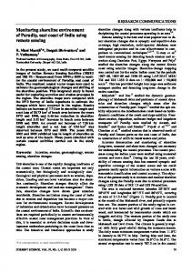
The unplanned growth of settlements along shorelines and the natural dynamics of coastal regions can have serious effects on the nature of an area’s coastal erosion. Monitoring and management of shorelines, therefore, are very important tasks, although they remain difficult to undertake. On the importance of shoreline monitoring, Di et al. (2003) states that shoreline mapping and shoreline change detection are critical for safe navigation, coastal resource management, coastal environmental protection, and sustainable coastal development and planning. Information about the high tide marks in association with the shoreline maps can be usefully in identifying areas of higher flood risk. With the historical cartographic documentation, it is possible to quantify the advance and retreat of the shoreline’s position, providing results that are very useful for the planning and management of costal zones. Boak and Turner (2005) brought the importance of shoreline variability to the attention of coastal scientists, engineers, and managers by recommending a functional definition of the shoreline, and also in pointing out that the challenge is to develop a sufficiently robust and repeatable technique to enable the detection of a chosen shoreline feature within the available data source. Shoreline monitoring is dependent upon the availability of economic support thereby necessitating a correct choice of a mapping technique. One form of shoreline mapping adopts the application of historical information to long-term analysis, and is always dependent on the uncertainties associated with the old data collection that normally comes from aerial photographs or topographic maps. Pajak and Leatherman (2002) showed the importance of accurate shoreline for mapping and management and explained that even for scientists and engineers experienced in the problems associated with identifying the correct position of shorelines using aerial

Goncalves, Awange and Krueger: GNSS-based monitoring and mapping of shoreline position in support of planning and management of Matinhos/PR (Brazil) 157

photos and the adverse effects of the inherent subjectivity, the spatial error involved in determining the historic shoreline positions may exceed the predicted rate of shoreline change. Furthermore, concerning shoreline historical data, there are some important requirements on error analysis and mapping accuracy that should be considered. For example, Crowell et al. (1991) indicate the importance of having a consistency in data application when computing coastal erosion rates. A challenge posed in attempting to achieve consistency in data is that of manipulating old data together with highly accurate new data for predicting shoreline positions. Modern techniques that attempt to address uncertainties in data include the application of geospatial approaches (see, e.g., Ahmad and Lakhan 2011). Of the geospatial approaches, the use of GIS has received quite an extensive coverage (see, e,g., Li, Weng and Willis 1998; Cracknell 1999; Kevin and El Asmar 1999; Green and King 2003; Hennecke et al. 2004; Liu and Jezek 2004; Schupp et al. 2005; Srivastava et al. 2005; Guariglia et al. 2006; Vanderstraete et al. 2006; Ekercin 2007; Sesli et al. 2009; Addo 2009; Pais-Barbosa et al. 2010; Ahmad and Lakhan 2011). For example, Li et al. (2001) describe a case study in Malaysia using aerial photos (taken at 5 year intervals) to map and monitor erosion while integrating the different data into a GIS. White and Asmar (1999) proposed the use of satellite images from Landsat Thematic Mapper (30 m spatial resolution) for monitoring and evaluating the rates of shoreline movement by comparing the positions of historical data points to identify areas of changes. Surveys with LiDAR involve the combination of the laser, a device that records the movements of the aircraft and GNSS receivers. LiDAR can make surveys in coastal areas with vertical accuracy 8-15 cm and a set of points spaced at least 1 m (without taking into account the processes of extraction shoreline). From those data the shoreline can be extracted and used in position analysis and also for obtaining the digital terrain models applied to coastal zones see e.g. Gorman et al. (1998), Gibeaut et al. (2001), and Awange and Kiema (2013, Chapter 24) . LiDAR data can also used to to identify vulnerable areas such as in the Queensland coasts and visualise the impacts of climate change, referring to the website http://www.longpaddock.qld.gov.au/coastalimpacts/impr ovedcoastalmapping.html. In comparison to GIS techniques, global navigation satellite systems (GNSS)-based techniques have not received wide coverage. Documented works on the applications of GNSS include, e.g., Ruggiero et al. (2005) who described shoreline monitoring by a variety of innovative surveying techniques, including real time kinematic global positioning systems (RTK-GPS) and

Goncalves et al. (2012) who compared the linear regression, robust parameter estimation, and neural network predictions models to predict the shoreline position in Brazil with the underlying data being from different kind of cartographic sources. In attempting to contribute towards GNSS-based shoreline monitoring methods, this paper describes a consistent, highly accurate, and low-cost method of shoreline monitoring that enables the evaluation of rates of short-term changes using relative kinematic GNSS positioning method. The study area is Matinhos coastal district of Brazil, an area where urban management has shown little concern about the position of the shoreline and its dynamical and local morphology (e.g., Soares et al., 1995). GNSS surveys were carried out in 2001, 2002, 2005, 2007 and 2008, and used to map the shoreline position. We organize the study as follows: Section 2 discusses the data collection (data source and study area) while section 3 presents the analysis method. The results are presented and analyzed in section 4, and the study concluded in section 5. 2.

Data Collection

2.1 Study area The study area for this work is located in Matinhos district of the state of Paraná, Brazil (approximate coordinates 25°49'00''S, 48°32'30''W, with an altitude of 3 m above sea level, see Fig. 1). According to IBGE (2010), the district of Matinhos with an area of 117 km2 is inhabited by approximately 29,428 people.

Figure 1: The study area, Matinhos District, Paraná State, Brazil 2.2 GNSS data collection To obtain a shoreline’s position and the water line using GNSS, the kinematic relative positioning mode of operation was adopted. For detailed discussion on this GNSS mode of operation, we refer to HofmanWellenhof et al. (2001, 2008), Seeber (2003), ElRabbany (2006), and Awange (2012). In this method, one receiver remains at the station whose position is precisely known (i.e., the base station in Fig. 2) while the other receiver (known as rover) moves to the features of interest (i.e., shoreline positions). Detailed discussion of

Goncalves, Awange and Krueger: GNSS-based monitoring and mapping of shoreline position in support of planning and management of Matinhos/PR (Brazil) 158

this approach can be found in the standard text books listed above. Using this method, surveys over a 6 km shoreline extension were carried out with the base station “PEDRA” (25º49’05,7799”S, 48º31’49,1364”W) located at “Matinhos Rock” shown in Fig. 2. The receivers at the base and roving stations were both set to collect data every 3 seconds at an elevation mask of 10º to minimize the influence of atmospheric and multipath errors (see, e.g., Awange 2012). Two crew manned the roving receivers along the shoreline, where one person started from Orquídas Street in the northern most point of the survey area while the other started from Londrina Street in the southern most point (Fig. 2). The surveys were stopped as soon as the two crew met somewhere in the middle of the observation area.

Figure 2: GNSS base station at Pedra and the start of rovers at Orquídas street in the North and Londrina street in the south During the surveys, the team endeavored to follow the same criterion in extracting the shoreline indicator. For example, in Fig. 3 (a) the shoreline was defined by the erosion scarp that can easily be seen in the boundary between the coast and ocean. For the case of Figure 3 (b), the shoreline was defined by the landward edge of shore protection structure. Also, in this study, the seaward stable dune vegetation line was used as an indicator of shoreline. The collected data was later post-processed using Ashtech Solutions 2.6 software, from which decimeter-level accuracy for shoreline positioning was achieved using relative kinematic positioning. The water line was observed at high and low tides, in accordance with the tidal predictions provided by the

(a) (b) Figure 3: Shoreline definition: (a) the shoreline is defined as erosion scarp, while in (b) it is the landward edge of shore protection structure. Center of Ocean Studies (CEM) at Federal University of Parana, the objective being to plan the best time to undertake the surveys. Fig. 4 shows an example of water levels reaching high tide on 13/09/2008. The high tide was between 12h00 and 15h00 and the survey was done between 12h34 and 13h43. The low tide was mapped on 14/09/2008, where it was expected between 6h00 and 9h00. The survey for this case was done between 06h54 and 07h54. In these tidal surveys, the line followed was the furthest point to which the waves reached. In some parts, the high-tide mark was equal to the shoreline.

Figure 4: (a) Predictions of the occurrence time for the high and low tides on 13/09/2008 (source: CEM (2008) http://www.cem.ufpr.br/mares.htm), (b) line of the high tidal survey, (c) water line survey, and (d) Line of the low tidal survey. 3.

Analysis Method

The analyses of the advance and retreat of the shoreline was done using the 2001 shoreline position as a reference, which was the time of the first GNSS shoreline survey. First, using the AutoCad software, the required shorelines (i.e., the reference 2001 shoreline and the one whose motion is desired) are selected and a visual inspection performed to determine if any change exist between lines.

Goncalves, Awange and Krueger: GNSS-based monitoring and mapping of shoreline position in support of planning and management of Matinhos/PR (Brazil) 159

If a positional change in a location is identified, then the software is used to mark at least 3 pairs of points that identify the perpendicular distance between the shorelines. An example is shown in Fig. 5 for the case of identifying shoreline movement between 2001 and 2005. Along a 70 m segment of shoreline, 5 pairs of points are marked and the distances between them stored. From such values, the mean and standard deviation of shoreline movement along this specific 70 m segment can be determined.

materials, a geometric correction of the IKONOS image was done to fit it with the map (note: all maps used in this work are in the WGS-84 datum, which is the system used by GPS and also by the Brazilian Directory of Hydrographic and Navigation (DHN) for their nautical charts). Field measurements and photographs were taken to allow features in the maps and IKONOS image to be identified. For example, Fig. 7 shows how photographs enabled features to be better identified on the thematic map, i.e., vegetation, a bicycle path, pavement road, the shoreline and foot path.

Figure 5: An example of identifying shoreline movement between 2001 and 2005 for a 70 m segment of coastline The length of the shoreline analyzed in this study is 6 km which was divided into 5 sectors in accordance with the similarity of identifiable features. Fig. 6 shows the sectors into which the study area was divided, with the extension of each sector and the principal thematic features listed in Table 1. A thematic map was developed from field observations to allow features near the coast to be identified. To recognize the features and create the thematic map, we used a satellite image (from the IKONOS spacecraft) of the study area and a vector file with the squares of the district, all plotted in a map. Before using these

Figure 6: The manner in which the study area was subdivided into sectors In addition, as examples, Fig. 7 and 8 show the parts of the thematic map for sectors I and II, respectively. As can be seen, Fig. 7 is an example where the current highwater mark and shoreline coincide, indicative of a greater potential for erosion. On the other hand, Fig. 8 shows a section of the coast where the shoreline and high-water mark do not coincide and also there is a vegetation line used as a shoreline indicator.

Table 1: The extent of the coastal sectors that make up the study area, and the most important thematic features. Sector I II III IV V

Extension (m) 1300 1900 700 700 1300

Features vegetation - foot path - bicycle path - pavement road riprap- road with problems of erosion vegetation with dunes - sediments - sand road sediments - foot path with problems of erosion – riprap vegetation -riprap - bicycle path - pavement road – grass

Goncalves, Awange and Krueger: GNSS-based monitoring and mapping of shoreline position in support of planning and management of Matinhos/PR (Brazil) 160

Figure 7: The part of thematic map of the study area, covering sector I

Figure 8: The part of thematic map of the study area, covering sector II. and III do the shoreline and high-tide lines coincided, while for the other sectors (II, IV and V) both lines 4. Results and Analysis coincided in many locations. This indicates that the ocean is eroding the coastline along sectors II, IV and V, 4.1 Comparison between the 2008 shoreline and causing damage to the streets and other constructions. high-tide line In Table 2, we list the mean distances between the 2008 An example is shown in Fig. 9, which shows an area in shoreline and high-tide line for each sector (I to V, see sector IV where during high tide some constructions Figure 7), as well as the maximum and minimum along the shore were being directly affected by the distances. The first point is that nowhere along sectors I ocean.

Goncalves, Awange and Krueger: GNSS-based monitoring and mapping of shoreline position in support of planning and management of Matinhos/PR (Brazil) 161

Table 2: Distance (in meters) between shoreline (SL) and high tide line water (HTLW) Minim Maxim Mean Extension of Extensi Exten um um of sector Sect on of sion distanc distanc the with or the Analy e e sample coincidence sector zed HTLW HTLW s HTLW-SL -SL -SL I 1300 1300 2.62 22.55 11.15 0 II 1900 985 3.61 13.76 7.21 915 III 700 700 11.61 42.34 26.76 0 IV 700 245 16.68 36.37 26.94 455 V 1300 525 8.02 27.07 15.52 775

4.2 Sector Analysis Maps to document the advance and retreat of shoreline were produced with respect to the sectors. The methodology applied to generate the results is described in some detail below, where the changes in shoreline location between 2001 and 2002 in Sector II, are used as an example. For the other sectors and years, only the results are presented. Table 3 represents a summary for sector I, where it is possible to observe the maximum advance of 9.53 m advance in 1300.00 m of extension between the years 2001-2005, and the maximum retreat of -4.29 m taking as reference the years 2001-2008 in 15 m of extension. Fig. 10 represent the plotted data of Table 3, the number 0.00 means no significant change between the comparisons in analysis in this sector. It can be seen that between 2001 and 2002, the shoreline advanced while from 2001 to 2005, the shoreline retreated. Table 3: Summary of the displacement of the shoreline for those segments of the coast along Sector I that experienced advancing or retreating shorelines. Vectors 1

Interval of time (years) 2001-2002

2 Figure 9: An image from sector IV (2008) showing how storm directly impacts upon urban infrastructure.

3 4 5

Mean shoreline movement - Sector I 20012002

20012005

9.53

20012008 6.41

4.91

0.00 1

0.00 2

3

4

5

6

7

8

-2.15 -3.82

-4.29

Figure 10: Mean Shoreline movement – Sector I

2001-2007

6 7 8

20012007

2001-2005

2001-2008

Extension Shift (m) analyzed (m) 0.00

0.00

50.00

-2.15

1300.00

9.53

0.00

0.00

730.00

4.91

38.00

-3.82

705.00

6.41

15.00

-4.29

Fig. 11 shows the extent (1900 m) of Sector II that has been divided into a number of segments or vectors, within which a number of pairs of points are selected to enable the amount of shoreline movement to be defined. Table 4 shows the values of shoreline movement inferred from these points, including the means, standard deviations, velocities (m/year) and extent of the vectors, with the results summarized in Table 5. Based on the results outlined in Table 5, it can be stated that a process of shoreline advancement occurred between 2001 and 2002 over 1264 m of the 1900 m of shoreline examined, representing 66.5% of this sector. During this time, the shoreline advanced with a mean velocity of 5.2 m/year, although over a 40 m long vector of this sector, the shoreline retreated at a rate of 4.73 m/year. Similarly to Table 5, we present the shoreline movement between the years 2001 and 2005, 2007 and 2008 in Tables 6 to 8, respectively. For the years 2001 to 2005

Goncalves, Awange and Krueger: GNSS-based monitoring and mapping of shoreline position in support of planning and management of Matinhos/PR (Brazil) 162

(Table 6), a retreat of 5.5 m over the 4 year period occurred over a 80 m long vector of shoreline. However, the shoreline appeared to be advancing over ca. 50% of Sector II (i.e., 955 m), at an average velocity of 4.7 m/year. What should be noted is that for the 2001 to 2005 analysis, 10 vectors were defined, showing that the shoreline behavior is not necessarily linear, and a significant amount of spatial and interannual variability is to be expected. Considering now the analyses for 2001-2007 (Table 7), over an extent of 505 m over Sector II, there was a mean shoreline advance 4.72 m, although there was also shoreline retreat of 3.08 m over a length of coast of 140 m. For the period between the years 2001 and 2008 (Table 8), there are a mean advance of 4.30 m over a length of coastline of 675 m, with shoreline retreat of 6.3 m over a 80 m length of coast. These results are summarized by Table 8, where the average values of the segments of Sector II coastline that advanced or retreated are listed, and visualized in columns in Figure 13. The appearance of such shoreline movement in reality is shown in Fig. 13, which shows the advance of shoreline in 2008 compared to 2001. Note the placement of riprap along the shore as an attempt to reduce the erosive action of the ocean. Through the relatively simple analysis shown here, one can still identify problems that may arise in infra-structure and coastal erosion, as seen in Figure 14, which shows how a bicycle path was destroyed by ocean action due to the advancing shoreline.

Figure 11: Collecting samples over the 1900 m of segment II that is divided into a number of portions.

Table 4: The results of the analysis of the shoreline movement from 2001 to 2002 for Sector II (see Figure 12). Part 1 Shift Part 2 Shift Part 3 Shift Advance 3.77 Advance 7.34 Advance 4.46 3.60 7.33 4.86 3.16 6.08 4.15 velocity 3.48 (m/year) 6.92 5.70 velocity standard velocity (m/year) 3.50 deviation 0.72 (m/year) 4.79 standard extension standard deviation 0.26 analyzed 54.0 deviation 0.67 extension extension analyzed 50.0 analyzed 60.0 Part 4 Shift Part 5 Shift Part 6 Shift Advance 3.66 Retreat 4.06 Advance 4.70 3.30 5.24 5.20 3.18 4.90 8.40 velocity 3.28 (m/year) 4.73 6.54 standard 4.60 deviation 0.61 7.72 extension 2.64 analyzed 70.0 8.68 3.36 7.58 4.01 4.02 3.73 7.03 5.27 8.14 6.95 9.37 5.21 8.92 3.95 6.81 3.39 4.90 velocity (m/year) 4.04 6.43 standard deviation 1.13 7.04 extension analyzed 470.0 5.09 4.84 4.46 8.41 7.05 8.47 velocity (m/year) 6.81 standard deviation 1.64 extension analyzed 630.0

Goncalves, Awange and Krueger: GNSS-based monitoring and mapping of shoreline position in support of planning and management of Matinhos/PR (Brazil) 163

Table 5: Comparison in the change of the shoreline locations for Sector II between (2001 and 2002) Mean Standard Vector Extension analyzed shift deviation v1 50 3.50 0.26 v2 54 6.92 0.72 v3 60 4.79 0.67 v4 470 4.04 1.13 v5 40 -4.73 1.24 v6 630 6.81 1.64 mean of shifting (velocity (m/year) extension (m) Advan ce 5.21 1264.00 Retrea t -4.73 40.00 Table 6: Comparison in the change in the shoreline locations for Sector II between (2001 and 2005) Mean Standard Vector Extension analyzed shift deviation v1 70 4.12 0.21 v2 60 1.93 0.58 v3 265 4.33 1.07 v4 55 2.62 0.94 v5 30 6.47 0.33 v6 100 4.92 1.24 v7 80 -5,53 0.69 v8 160 5.24 0.62 v9 150 5.42 0.27 v10 65 7.03 1.57 mean of shifting (velocity (m/year) extension (m) Advan ce 4.68 955.00 Retrea t -5,53 80.00

v7 v8 v9 v10

Advance Retreat

5.23 4.46 3.69 4.92

0.91 0.53 1.31 0.48 extension (m) 505.00 140.00

Table 8: Comparison in the change in the shoreline locations for Sector II between (2001 and 2008) Mean Standard Vector Extinction analyzed shift deviation v1 145 2.86 0.96 v2 50 4.87 1.16 v3 80 4.21 0.94 v4 40 3.54 0.32 v5 80 -6.30 1.03 v6 150 5.72 1.26 v7 80 4.16 0.91 v8 80 3.54 0.79 v9 50 5.46 0.56 mean of shifting (velocity (m/year) extension (m) Advance 4.30 675.00 Retreat -6.30 80.00 Table 9: Summary of the displacement of the shoreline for those segments of the coast along Sector II that experienced advancing or retreating shorelines. Vectors 1

Interval of time (years) 2001-2002

2 3

2001-2005

4 5

Table 7: Comparison in the change in the shoreline locations for Sector II between (2001 and 2007) Mean Standard Vector Extension analyzed shift deviation v1 50 1.75 0.34 v2 10 -4,71 0.78 v3 55 6.36 0.97 v4 30 4.23 0.25 v5 40 4.17 1.17 v6 80 -6,29 1.47

150 90 90 50 mean of shifting (velocity (m/year) 4.72 -3,08

2001-2007

6 7 8

2001-2008

Extension analyzed (m)

Shift (m)

1264.00

5.21

40.00

-4.73

955.00

4.68

80.00

-5.53

505.00

4.72

140.00

-3.08

675.00

4.30

80.00

-6.30

Goncalves, Awange and Krueger: GNSS-based monitoring and mapping of shoreline position in support of planning and management of Matinhos/PR (Brazil) 164

Mean shoreline movement Sector II 20012002

5.21

20012005

20012007

4.72

4.68

20012008 4.30

Table 10: A summary of the displacement of the shoreline for those segments of the coast along Sector III that experienced advancing or retreating shorelines. Vectors 1

Interval of time (years)

Extension analyzed (m)

Shift (m)

90.00

6.55

215.00

-12.34

190.00

17.32

275.00

-15.89

140.00

12.34

320.00

-13.5

70.00

11.09

320.00

-13.5

2001-2002

2 3

2001-2005

4 5

2001-2007

6 1

2

3

4

5

6

7

8

7

2001-2008

8 -3.08 -4.73

-5.53

Fig. 14 shows the mean shoreline movement for sector III with cases of retreat of shoreline with the variation between -12.34 m and -15.89 m and advance variations between 6.55 m and 17.32 m. -6.30

Figure 12: Schematic diagram showing the relative displacement of the shoreline in Sector II between 2001 and 2008.

Mean shoreline movement Sector III 2001-2 002

20012005

2001-2 007

17.32

12.34

20012008 11.09

6.55

1

Figure 13: An example of how shoreline advancement causes damage to urban infrastructure, shown here by the damaged bicycle path. Results for sectors III, IV and V are summarized in Tables (10, 11, 12), with the corresponding Figs. (14, 15, 16) providing column graphics for analysis. In Table 10 shows that for Sector III a retreat of -12.34 m for 215.00 m of extension for the years of 2001 -2002, -15.89 m for 275.00 m of extension for the year 2001 – 2005 and 13.50 m for the years 2001-2007 and 2001-2008 with the extensions of 320.00 m each is observed.

2

3

4

-12.34 -15.89

5

6

-13.5

7

8

-13.5

Figure 14: Mean Shoreline movement – Sector III Table 11 shows some stable cases of shoreline between the analysis for 2001-2005 and no detection of advance between of 2001-2007.

Goncalves, Awange and Krueger: GNSS-based monitoring and mapping of shoreline position in support of planning and management of Matinhos/PR (Brazil) 165

Table 11: A summary of the displacement of the shoreline for those segments of the coast along Sector IV that experienced advancing or retreating shorelines. Vectors

Interval of time (years)

Extension Shift (m) analyzed (m)

1 2

2001-2002

3 4

2001-2005

5 6

2001-2007

7 8

2001-2008

17. Table 13 shows the summary of the velocity along Sectors I to V. In the comparison between 2001 and 2008, sector II is seen to have the highest velocities of 6.76 m/year for advances and -7.89 m/year for retreat. Table 12: Summary of the displacement of the shoreline for those segments of the coast along Sector V that experienced advancing or retreating shorelines

200.00

9.34

50.00

-6.51

170.00

12.08

0.00

0.00

0.00

0.00

80.00

-11.47

2

0.00

0.00

3

255.00

-7.41

Fig. 15 shows the overview for sector IV with the maximum of reatreat of -11.47 m between the years of 2001-2007.

Vectors

Interval of time (years)

1

Extension analyzed (m)

Shift (m)

0.00

0.00

0.00

0.00

85.00

4.21

315.00

-4.99

0.00

0.00

435.00

-7.09

0.00

0.00

540.00

-7.61

2001-2002 2001-2005

4 5

2001-2007

6 7

2001-2008

8

Mean shoreline movement - Sector IV 20012002

20012005

20012007

12.08

20012008

9.34

Mean shoreline movement - Sector V 20012002

20012005

20012007

20012008

4.21

0.00 0.00 1

2

3

4

5

0.00 6

-6.51

7

0.00 0.00 8

1

2

0.00 3

4

5

0.00 6

7

8

-7.41 -11.47

-4.99 -7.09

Figure 15: Mean Shoreline movement – Sector IV In Table 12 and Fig. 16, we visualized the analysis for sector V. Note that this sector presents problems in the infrastructure due to the retreat of the sea that occurred since 2005. To a large extent this passage is remarkable as it shows the presence of sidewalks destroyed, and in some places, the erosion reaches out to the street. When the value 0.00 is found in the table it doesn´t necessary mean that there is no problem of infrastructure, but in most of cases this indicate that the shoreline does not have natural space for its movement like shown in Fig.

-7.61

Figure 16: Mean Shoreline movement – Sector V

Goncalves, Awange and Krueger: GNSS-based monitoring and mapping of shoreline position in support of planning and management of Matinhos/PR (Brazil) 166

Figure 17: Sector V infrastructure problems. Table 13: Summary of the velocities (m/year; 2001 and 2008) of the shoreline along Sectors I to V that experienced advancing or retreating shoreline.

Sector Advance Reatreat 5.

I 2.98 -1.46

II 2.70 -2.81

III 6.76 -7.89

IV 3.06 -3.63

V 0.60 -2.81

Conclusion

This paper has presented an example of how GNSS techniques (in this case the relative kinematic GPS method) can be used to monitor the advance or retreat of coastal areas. The area of interest, the district of Matinhos, Brazil, is experiencing damage to infrastructure from ocean erosion arising from advancing or retreating shoreline. Five GPS surveys were carried out in 2001, 2002, 2005, 2007 and 2008. Relative positions of the shoreline and high-tide mark were mapped and changes in the shoreline defined over one sector of the coastline. The result was a series of thematic maps that are useful to urban planning and coastal management authorities as they provide tools for monitoring. In the study area, it was found that tendencies towards shoreline advance were more prominent than retreat. Zones where the shoreline coincides with the high-tide mark were identified, and in fact in some case, these lines are in direct contact with engineering constructions. Hence, the resulting maps show areas where the coast may be expected to suffer erosion in the event of storms. However, this is not to say that the shoreline will continue to advance over time, with the additional need for more historical data and a longer-term period of observation being important to reach and obtain more accurate conclusions and predictions. GNSS-based method thus offers a quicker, all-weather, highly accurate and continuously updatable shoreline positional time series relevant for monitoring and management tasks undertaken by engineers and coastal authorities. Its

disadvantages, however, is that it is only limited to small monitoring regions such as the case of Brazil considered in this contribution. For the countries such as Australia with very long coastal lines, the application of GNSSbased approach faces challenges of being time consuming and may require high manpower thus increasing the costs. Also, depending on coastal characteristics, e.g., of escarpment and mangrove trees, data collection using GNSS could be impracticable. In such cases, other techniques such as LIDAR come in handy. However, considering the case of Brazil where the cost of undertaking a GNSS shoreline monitoring is cost effective, the approach presented in this contribution suffices. Acknowledgments Rodrigo Mikosz and Claudia Krueger acknowledges the support of CNPq – Brazil and also for the students of Cartographic Engineering at UFPR who worked in the project and in field to support the geodetic surveys in Matinhos District between them are Ruth da Maia, Sibele Mazur and Nassau Nardez. References Addo, K. A. (2009), Detection of coastal erosion hotspots in Accra, Ghana. Journal of Sustainable Development in Africa 11(4): pp.253–265. Ahmad, S. R. and Lakhan, I. L. (2012), GIS-based analysis and modeling of coastline advance and retreat along the coast of Guyana. Marine Geodesy, 35: pp.1-15. Awange, J. L and Kiema JBK., (2013), Environmental Geoinformatics – monitoring and management, Springer, in press. Awange, J. L., (2012), Environmental monitoring using GNSS Global Navigations Satellite Systems, Springer, 382pp. Boak, E. H. and Turner, I. L. (2005), Shoreline definition and detection: A Review. Journal of Coastal Research. 21 (4), pp.688-703. Cracknell, A. P. (1999), Remote sensing techniques in estuaries and coastal zone—an update. International Journal of Remote Sensing 19(3): pp.485–496. Crowell, M., Letherman, S. P. and Buckley, M. K. (1991), Historical shoreline change: error analysis and mapping accuracy. Journal of Coastal Research, 7 (3), pp.839-852.

Goncalves, Awange and Krueger: GNSS-based monitoring and mapping of shoreline position in support of planning and management of Matinhos/PR (Brazil) 167

CEM - Center of Ocean Studies, Federal University of Parana. Predictions of the occurrence of high and low time. http://www.cem.ufpr.br/mares.htm (Accessed 10.09.2008). Di, K., R. Ma, Wang J., and Li R.. (2003), Coastal mapping and change detection using highresolution IKONOS satellite imagery. ACM InternationalConference Proceeding Series, Vol. 130, Proceedings of the 2003 annual national conference on digital government research, pp. 1–4. Boston, MA: Digital Government Society of North America. El-Rabbany, A. (2006), Introduction to GPS global positioning system, 2nd edn. Artech House, Boston. Ekercin, S. (2007), Coastline change assessment at the Aegean sea coasts in Turkey using multitemporal Landsat imagery. Journal of Coastal Research 23(3): pp.691–698. Gibeaut, J. C., Hepner T., Waldinger R., Andrews J., Gutierrez R., Tremblay T. A., Smyth R. and Xu L. (2001) Changes in gulf shoreline position, Mustang, and North Padre Islands, Texas. A report of the Texas Coastal Coordination Council pursuant to National Oceanic and Atmospheric Administration. Bureau of Economic Geology, The University of Texas, Austin Texas, pp. 30. Goncalves, R. M., Awange, J., Krueger, C. P., Heck, B., and Coelho, L. S. (2012), A comparison between three short-term shoreline prediction models. Ocean & Coastal Management. v. 69, pp. 102-110. Gorman L, Morang A, Larson R (1998) Monitoring the coastal environment; Part IV: mapping, shoreline changes, and bathymetric analysis. Journal of Coastal Research (14): 61-92. Green, D. R., and S. D. King. (2003), Progress in geographical information systems and coastal modeling: An overview. In Advances in coastal modeling, V. C. Lakhan (ed.), pp. 553–580. Guariglia, A., A. Buonamassa, A. Losurdo, R. Saladino, M. T. Trivigno, A. Zaccagnino, and A. Colangelo. (2006), A multisource approach for coastline mapping and identification of shoreline changes. Annals of Geophysics, 49(1): pp.295–304. Hennecke, W. G., C. A. Greve, P. J. Cowell, and B. G. Thom. (2004), GIS-based coastal behavior modeling and simulation of potential land and property loss: Implications of sea-level rise at Collaroy/Narrabeen Beach, Sydney (Australia). Coastal Management 32(4): pp. 449–470.

Hofman-Wellenhof B, Lichtenegger H. and Colins J. (2001), Global positioning system: theory and practice, 5th edn. Sprienger, Wien. Hofman-Wellenhof B, Lichtenegger H., and Wasle E. (2008), GNSS global navigation satellite system: GPS, GLONASS, Galileo and more. Sprienger, Wien. IBGE – (Brazilian Institute of Geography and Statistics) – Data banking of the cities. http://www.ibge.gov.br/cidadesat/default.php. (Accessed 06.08.2008). Kevin, W. and El Asmar H. M. (1999), Monitoring changing position of coastlines using thematic mapper imagery, an example from the Nile Delta. Geomorphology 29: pp.93–105. Li, R., Di, K., Ma, R. (2001), A comparative study of shoreline mapping techniques. In: The 4th International Symposium on Computer Mapping and GIS for Coastal Zone Management, Proccedings, Nova Scotia, pp. 18-20. Li, R., K. C. Weng and D. Willis. (1998), A coastal GIS for shoreline monitoring and management—case study in Malaysia. Surveying and Land Information Systems 58(3): pp.157–166. Liu, H. and K. C. Jezek. (2004), Automated extraction of coastline from satellite imagery by integrating Canny edge detection and locally adaptive thresholding methods. International Journal of Remote Sensing 25(5):937–958. Pajak, M. J. and Leatherman, S. (2002). The high water line as shoreline indicator. Journal of Coastal Research 18 (2): pp.329-337. Pais-Barbosa, J., Veloso-Gomes F., and Taveira-Pinto F.. (2010), GIS tool for coastal morphodynamics analysis. In Coastal and marine geospatial technologies, D. R. Green (ed.), pp. 275–283. The Netherlands: Springer. Ruggiero P., Kaminsky, G.M., Gelfenbaum, G. and Voigt B., (2005), Seasonal to interannual morphodynamics along a high-energy dissipative litorral cell. Jornal of Coastal Research, n.22, pp. 553-578. Schupp, C. A., E. R. Thieler, and J. F. O’Connell. (2005), Mapping and analyzing historical shoreline changes using GIS. In GIS for coastal zone

Goncalves, Awange and Krueger: GNSS-based monitoring and mapping of shoreline position in support of planning and management of Matinhos/PR (Brazil) 168

management, D. Bartlett and J. Smith (ed.), pp. 219– 228. Boca Raton, FL: CRC Press.

Hurghada, Egypt. International Journal of Remote Sensing 27(17): pp.3645–3655.

Seeber, G. (2003), Satellite Geodesy - Foundations, Methods, and Applications. Walter de Gruyter. Berlin, New York, pp.589.

White, K.; Asmar, E. L. (1999), Monitoring changing position of coastlines using thematic mapper imagery, an example from the Nile Delta. Geomorphology, v. 29, pp. 93-105.

Sesli, F. A., F. Karsli, I. Colkesen, and N. Akyol. (2009), Monitoring the changing position of coastlines using aerial and satellite image data: An example from the eastern coast of Trabzon, Turkey. Environmental Monitoring and Assessment 153(1–4): pp.391–403. Soares, C. R., Vobel, I., Paranhos Filho, A. C. (1995), The marine erosion problem in Matinhos municipality. In: Land Ocean Interactions on the Coastal Zone, São Paulo, pp.48-50. Srivastava, A., Niu, X., Di, K. and Li, R.. (2005), Shoreline modeling and erosion prediction. Proceedings of the ASPRS 2005 Annual Conference, March 7–11, Baltimore, Maryland. Vanderstraete, T., R. Goossens, and Ghabour T. K. (2006), The use of multi-temporal Landsat images for the change detection of the coastal zone near

Biography Rodrigo Mikosz Gonçalves graduated in Cartographic Engineering at Federal University of Parana (UFPR), Brazil (1999), MS in Electrical Engineering and Industrial Informatics by Technological Federal University of Parana (UTFPR), Brazil (2004) and Ph.D. in Geodetic Sciences, UFPR with research period at Karlsruhe Institute of Geodesy, Karlsruhe Institute of Technology (KIT), Germany (2010). He is currently adjunct professor of Federal University of Pernambuco (UFPE), Brazil and permanent member of the PostGraduation Program in Geodetic Sciences and Technologies Geoinformation. He has experience in the field of geodesy, acting on the following topics: coastal mapping, monitoring and modeling of temporal geodetic data.