Goldberg, R. G. "Quantization and Waveform Coders". A Practical Handbook of
Speech Coders. Ed. Randy Goldberg. Boca Raton: CRC Press LLC, 2000.
Goldberg, R. G. "Quantization and Waveform Coders" A Practical Handbook of Speech Coders Ed. Randy Goldberg Boca Raton: CRC Press LLC, 2000
© 2000 CRC Press LLC
Chapter 7 Quantization and Waveform Coders
The goal of quantization is to accurately encode data using as little information (as few bits) as possible. Efficient and accurate parameter quantization is central to speech coding because pertinent information must be represented as accurately as the coding requirements dictate using as little information as possible. Quantization can be applied directly to a sampled speech waveform or to parameter files such as the output of a vocoder analysis. Waveform coders encode the shape of the time-domain waveform. Basic waveform coding approaches often do not exploit the constraints imposed by the human vocal tract on the speech waveform. As such, waveform coders represent nonspeech sounds (music, background noise) accurately, but do so at a higher bit rate than that achieved by efficient speech-specific vocoders. Vector quantization (VQ) encodes groups of data simultaneously instead of individual data values. Advances in vector quantization of line spectral frequencies (LSFs) is one of the primary reasons for improved speech quality in leading low bit-rate coding schemes. This chapter covers basic quantization of single element data and various waveform coding approaches. VQ is presented along with the computation reduction techniques that make it practical. The chapter concludes with a description of current approaches for efficient quantization of LSFs.
2000 CRC Press LLC
7.1
Uniform Quantization
The simplest type of quantization is uniform, or linear, quantization. The range of values for the signal is segmented into evenly spaced quantization levels. The number of levels is equal to the number of codewords available for quantization. If the capacity of n bits is used, there are 2 n codewords available and 2n quantization levels. A codeword directly represents a quantized level of the signal.
7.1.1
Uniform Pulse Code Modulation (PCM)
When uniform quantization is applied directly to an audio waveform, the process is called pulse code modulation (PCM). Pulse code modulation is the simplest method of speech coding and is essentially the sampling process as discussed in Section 3.1. An analog speech signal is sent into an anti-aliasing analog lowpass filter which eliminates all frequencies above half the sampling rate. The signal is then sent through an analog-to-digital (A/D) converter which converts the signal to a sequence of numbers, with the time distance between sample points equal to the sampling rate. The signal, now a sequence of numbers, can be stored or sent through a digital transmission channel. The PCM analysis process is displayed in Figure 7.1. The input signal is an analog signal, typically a varying voltage level in an analog circuit. The lower plot of the input signal represents the continuoustime frequency domain of the input speech. The second plots (time domain upper, frequency domain lower) display the continuous-time impulse and frequency responses, respectively, of the analog low-pass filter. The input speech is bandlimited by the lowpass filter with the result displayed in the third plots. The bandlimited analog signal is sampled at discrete time intervals to produce the last plots. The samples are shown as the dots on the time domain waveform. The frequency domain plot indicates the cyclical nature of the Fourier representation of a discretely sampled signal. To reconstruct the analog signal, the digital signal is passed through a Digital-to-Analog (D/A) converter and then filtered by a simple low-pass interpolating analog filter which generally has the same characteristics as the anti-aliasing pre-filter that was used to filter the original analog signal. A representation of the PCM reconstruction process can be seen in Figure 7.2. The discretely sampled signal is converted to the
2000 CRC Press LLC
FIGURE 7.1 Time- and frequency-domain representations of signals at different stages during pulse code modulation (PCM) analysis.
pulse-type waveform of the second plots. This waveform has higher harmonics not present in the original signal. The lowpass filter removes these unwanted higher frequencies. PCM is a simple coding scheme and is often used when transmission bandwidth (or storage space) is not a limitation. PCM is more susceptible to bit errors than other speech waveform coding methods such as delta-modulation [79], because a single bit error can change a value from the positive maximum value to the minimum value possible. Therefore, if speech quality is important in a noisy transmission environment, PCM is not desirable even if the coding bit rate is not an issue. The reconstruction error (the difference between the original signal and the reconstructed signal) is affected by quantization error that is introduced in the PCM coding scheme. This error is introduced during the process of analog-to-digital conversion. In order to represent a signal digitally, the values of the signal must be approximated to the
2000 CRC Press LLC
FIGURE 7.2 Time- and frequency-domain representations of signals during pulse code modulation (PCM) reconstruction.
closest possible discrete values. For example, if the A/D converter represents each value with only 3 bits, then the dynamic range of the signal is sectioned into 8 even parts and each sample is represented by the closest match. For a signal that fluctuates through the range of [-1V to 1V], its (dynamic range) is represented by the values: [-7/8 -5/8 3/8 -1/8 1/8 3/8 5/8 7/8]. The quantization error introduced by a 16 bit D/A converter is generally not perceptible to the human ear. For a speech signal that may contain some pure silence, one may choose a quantization scheme that contains zero as a quantization value, so that quantization noise is not introduced when no signal is present. This can be accomplished by shifting the values by 1/2B in either direction where B is the number of bits per sample used in quantization. In the above example, the quantization values shift to [-1 -3/4 -1/2 -1/4 0 1/4 1/2 3/4]. The only issue with this scheme is that it is not symmetric: -1 V is represented, but 1V must be approximated by 3/4 V.
2000 CRC Press LLC
7.2
Nonlinear Quantization
It is often beneficial to use nonlinear spacing between the quantization levels. The spacing of the quantization levels can be set based on the distribution of sample values in the signal to be quantized. The distance between adjacent quantization levels is set smaller for regions that have a larger share of the sample values. When adjusted in this manner, the overall quantization error is smaller. In direct speech waveform coding, logarithmically spaced quantization levels are used to best match the expected distribution of the speech signal.
FIGURE 7.3 Distribution of quantization levels for a nonlinear 3-bit quantizer.
Figure 7.3 shows the distribution of quantization levels for a nonlinear 3-bit quantizer. The input value S is positioned on the x-axis, and the corresponding output value is S' on the y-axis. Although only four levels are shown, the same logarithmic scale is used for negative S, where the third bit indicates the sign of S and S'.
2000 CRC Press LLC
7.2.1
Nonuniform Pulse Code Modulation
Nonuniform pulse code modulation works similarly to PCM except that the quantization values are nonlinearly distributed through the dynamic range. Schemes employ fine quantizing steps around frequently occurring values, and course step sizes around the more rarely occurring values. An alternative view is to mimic the human ear and distribute the bits so that the quantization noise is less perceptible. µ -law and A-law coders fall under the latter of these methods. They are both quasi-logarithmic in that they are linear for small signal values and logarithmic for large signal values. The formula for A-law companding (compressing/expanding) is: x 1 Alogx A sgn( x ); 0 ≤ x ≤ A1 + e max c( x ) = x 1+ log e ( A x / x max ) 1 sgn( x ); A < xmax ≤ 1 x max 1+ log e A
(7.1)
where the signal x has the dynamic range: −x max ≤ x ≤ x max , A ≥ 1, and sgn(x) represents the sign of x. The formula for µ-law companding is: c( x ) = x max
log e (1+ µ x / x max ) log e (1+ µ )
( sgn )( x );
µ≥0
(7.2)
A-law companding is used in European telephony (the European PCM standard) with A=87.56. North American telephony employs µ-law companding (The North American PCM standard) with µ=255. The A-law and µ-law standards are specified in the International Telecommunications Union (ITU) recommendation G.711 [186]. Figure 7.4 plots companding functions for A-law and µ-law for different values of A and µ. The bottom plot highlights the difference between the North American and European standards. As can be seen, the two are essentially the same, differing only slightly for very small input values.
7.3
Differential Waveform Coding
A coder that quantizes the difference waveform rather than the original waveform is called differential pulse code modulation (DPCM). Ei-
2000 CRC Press LLC
FIGURE 7.4 Companding functions for A-law and µ-law for different values of A and µ. The bottom plot indicates the difference between North American and European standards.
ther linear or nonlinear quantizers can be used in DPCM systems. Firstorder or higher-order predictors can also be used to enhance DPCM performance. The linear delta modulation quantization scheme is also a type of DPCM coder. As mentioned above, PCM, both uniform and nonuniform, is quite susceptible to bit errors. If one of the more significant bits is erroneously reversed, the representation of that sample will be drastically off. Differential waveform coders such as differential pulse code modulation (DPCM) and delta modulation produce less perceptual error for single bit errors. These coders encode the difference signal (the difference between adjacent samples) rather than the original signal. These methods yield poor performance if the signal is completely random; however, because subsequent samples in speech signals are highly correlated, the difference signal generally has a smaller dynamic range than the origi-
2000 CRC Press LLC
nal signal. As such, quantizing the difference signal yields better coding quality than uniform PCM at the same bit rate.
7.3.1
Predictive Differential Coding
Predictors are often used in differential quantization to lower the variance of the difference signal. The smaller the variance of the coded signal, the better the quality of the coding that can be achieved with all other variables being equal. Predictive differential coding predicts the value of the present sample from the values of previous samples, and then encodes the difference between the predicted and actual sample values. The input to a quantizer of this type is the difference signal: d ( n) = x ( n) − ~ x ( n)
(7.3)
which is the difference between the unquantized input sample, x(n), and x (n ) . a predicted value of the input sample, ~ ~ If the prediction is accurate, then x (n) ≈ x(n) and the variance of the difference signal d(n) is smaller than the variance of the original signal x(n). A differential quantizer with a given number of levels yields a smaller quantization error than does quantization of the same highly correlated signal directly. x (n) is often calculated using linear prediction The predicted value ~ x (n) is a linear combination of the past p quantized (LP). That is, ~ values: x~( n ) =
p
∑ ak xˆ (n − k )
(7.4)
k =1
The optimal values (minimum prediction error) for lowpass filtered speech for up to fifth-order prediction are as follows: a = 0.86 a1 = 0.64 a 2 = 0.40 a 3 = 0.26 4 a 5 = 0.20
Values from[123]
These prediction coefficients are determined by performing LP analysis on long time durations (many minutes) of the speech signal that include a representative distribution of different speech sounds. See Chapter 4 for a description of LP analysis.
2000 CRC Press LLC
FIGURE 7.5 Delta modulation with 1-bit quantization and first-order prediction.
7.3.2
Delta Modulation
The simplest form of differential quantization is first-order, one-bit linear delta modulation. It has a single predictor (a1 = a = 1), so d (n) = x(n) − xˆ (n − 1)
(7.5)
The quantizer has only two levels (1 bit) and the step size is fixed. Each estimate of the signal xˆ ( n ) differs from the previous estimate xˆ ( n − 1) by only the step size δ. This method is used for signals with high sampleto-sample correlation, like highly oversampled speech waveforms. The coded output waveform is coded to 1 bit per sample with this simple quantizer. Linear delta modulation can use a quantizer with more than two levels, and the predictors can be of any order and need not be fixed to 1. A block diagram of a delta modulation system with 1-bit quantization and single-order prediction is shown in Figure 7.5, and Figure 7.6 illustrates the coding of a waveform. A single-bit codeword specifies if the next sample of the signal is greater than or less than the previous sample. A "1" designates that
2000 CRC Press LLC
FIGURE 7.6 Delta modulation (Two types of quantization noise).
the next sample is greater than the last, while a "0" represents that the next sample is less than the last. If the sample is determined to be greater than the last, then the next sample is represented by the last signal plus a fixed increment; conversely, when the next sample is determined to be less than the last, it is represented by the previous sample minus the same fixed increment. This fixed increment is represented by the symbol δ. Both the sampling rate and the step size δ need to be chosen properly for delta modulation to be effective. The coding error in delta modulation can be classified in two groups as shown in Figure 7.6. Slope overload occurs when the step size δ is not large enough to handle large sample-to-sample changes in the speech waveform. Granular noise occurs because the step size, δ, is too large to accurately narrow in on the speech waveform. Increasing δ would reduce slope overload distortion but increase granular noise. Conversely, decreasing δ reduces granular noise but increases errors due to slope overload. To reduce slope overload without affecting granular noise it is necessary to increase the sampling rate. For this reason delta modulation is often used on greatly oversampled signals.
2000 CRC Press LLC
7.4
Adaptive Quantization
The main tradeoff in signal quantization is making the quantization step size large enough to accommodate the maximum peak-to-peak range of the signal while keeping this step size small enough to minimize quantization noise. As discussed previously, nonlinear quantization addresses this problem in one manner. Another approach adapts the properties of the quantizer to the signal by having large quantizer step sizes in regions of the signal where the peak-to-peak range is high, and small step sizes when the peak-to-peak range is small, that is, to let the step size vary so that it matches the short-term variance of the input signal. Adaptive quantization schemes reduce the quantization error below that of µ-law quantization.
7.4.1
Adaptive Delta Modulation
Linear delta modulation can be modified so that the step size varies to better match the variance of the difference signal. The step size is increased or decreased when the output quantization code meets a predetermined criteria. An example of step size logic is as follows: • Increase the step size by a multiplicative factor, P > 1, if the present code word c(n) is the same as the previous code word c(n − 1), otherwise, decrease the multiplier by a multiplicative factor, Q < 1. This adaptation strategy is motivated by the bit patterns observed in linear delta modulation. Referring to Figure 7.6, it can be seen that the periods of slope overload are denoted by consecutive zeros or ones. Increasing the step size in these regions will reduce the slope overload. Periods of granularity are signaled by alternating codewords, and decreasing the step size minimizes quantization error in these regions.
7.4.2
Adaptive Differential Pulse Code Modulation (ADPCM)
When an adaptive step size is introduced into DPCM systems, the new quantization scheme is classified as an adaptive DPCM (ADPCM) system. Because the signal being quantized is a difference signal, ADPCM systems have predictors of first or higher order.
2000 CRC Press LLC
A simple but useful ADPCM system was introduced by Cummiskey, Jayant, and Flanagan in [25, 78]. The coder makes instantaneous exponential changes of quantizer step size, includes a simple first-order predictor, and has an adaptation strategy that depends only on the previous code-word. Figure 7.7 shows a block diagram of the coder. The signal is coded as follows: x ( n) δ ( n) = x ( n) − ~
(7.6)
The difference signal, δ(n), is calculated and uniformly quantized into δˆ ( n) with step size σ(n):
δˆ (n) = Qσ ( n ) [δ (n)]
(7.7)
The δˆ ( n ) value is encoded as the digital output, c(n). The step size σ(n) is then scaled by the multiplier, Mc(n), corresponding to c(n), to adapt the step size for the quantization of the next sample:
σ (n + 1) = M c ( n ) σ (n)
(7.8)
The multiplier, Mc(n), is selected by the "LOGIC" box in the diagram, where each code word corresponds to a different multiplier scaling of σ(n). Figure 7.8 shows the quantizer levels for a 3-bit coder. The difference signal, δ(n), is quantized to 0.5σ, for 0 < δ ≤ σ, and δ(n) is quantized to 1.5σ, for σ < δ ≤ 2σ, etc. For δˆ quantized as 0.5σ, the output codeword, c(n), is set to 100, and the corresponding multiplier is M00. (The value of the multipliers is not indicated in Figure 7.8. Multiplier symbols are displayed to show the tied correspondence to c(n).) The most significant bit indicates the sign of the coded output. Note that there are only four distinct multipliers because the sign of quantizer output (the most significant bit) is not utilized in the adaptation logic. The adaptation depends only on the magnitude of δˆ . The low-level multipliers, such as M00, are kept small (M00