Such a golden implementation is exploited for software development in several domains, including embedded software â a low resource- consuming version of ...
Golden Implementation Driven Software Debugging Ansuman Banerjee, Abhik Roychoudhury, Johannes A. Harlie, Zhenkai Liang National University of Singapore
{banerjee,abhik,johannes,liangzk}@comp.nus.edu.sg
ABSTRACT
1.
The presence of a functionally correct golden implementation has a significant advantage in the software development life cycle. Such a golden implementation is exploited for software development in several domains, including embedded software — a low resourceconsuming version of the golden implementation. The golden implementation gives the functionality that the program is supposed to implement, and is used as a guide during the software development process. In this paper, we investigate the possibility of using the golden implementation as a reference model in software debugging. We perform a substantial case study involving the Busybox embedded Linux utilities while treating the GNU Core Utilities as the golden or reference implementation. Our debugging method consists of dynamic slicing with respect to the observable error in both the implementations (the golden implementation as well as the buggy software). During dynamic slicing we also perform a stepby-step weakest precondition computation of the observable error with respect to the statements in the dynamic slice. The formulae computed as weakest pre-condition in the two implementations are then compared to accurately locate the root cause of a given observable error. Experimental results obtained from Busybox suggest that our method performs well in practice and is able to pinpoint all the bugs recently published in [8] that could be reproduced on Busybox version 1.4.2. The bug report produced by our approach is concise and pinpoints the program locations inside the Busybox source that contribute to the difference in behavior.
Software debugging can be an extremely time-consuming activity. It seeks to answer the following question - given a program P and a test input t which fails in P , how to explain the failure of t in P ? Debugging usually returns a bug report - a fragment of P that is highlighted to the programmer. We observe that debugging of a given test input in a buggy program can be aided by the presence of a golden implementation. This golden implementation captures how the buggy program is “supposed” to behave. The presence of such golden implementations are common in many domains, such as for embedded software (where the embedded software is derived as a low-resource consuming equivalent of a golden implementation) or for web-servers (where both the buggy and the golden implementations implement the HTTP protocol). It should be noted that the golden implementation often employs different data structures as compared to the program being debugged. To exploit the golden implementation in software debugging, the debugging method should be based on semantic analysis. Evolving programs (where the code of a program evolves from one version to another1 ) can be viewed as a special case of golden implementation — where the older version of an evolving program can be treated as a golden implementation. For evolving programs, the older version or golden implementation is quite similar (in terms of code) to the buggy implementation. In this paper, we study how the golden implementation can be effectively exploited for software debugging. Our method involves simultaneously performing dynamic slicing and symbolic execution in both the programs - the golden implementation as well as the buggy implementation. The slicing is performed with respect to the observable error, which is set as the slicing criteria. Moreover, given the specification of the observable error, we perform a step-by-step weakest pre-condition calculation along the dynamic slice. The resultant weakest pre-conditions accumulated in the two programs are then compared to find new / missing constraints accumulated in the buggy implementation. The lines of code contributing to these constraints form our bug report. We employ our methods on Busybox [2] — the de-facto standard for Embedded Linux devices. It provides many of the standard Linux utilities, but has a smaller code size (size of the executable) than the GNU Core Utilities, net-tools and procps. We choose two versions of Busybox, namely, version 1.4.2 and the latest version 1.16.0 and employ our methods to find the root causes of errors that have previously been reported in very recent literature [8]. In
Categories and Subject Descriptors D.2.5 [Software Engineering]: Testing and Debugging—Debugging aids, Symbolic execution; D.3.4 [Programming Languages]: Processors—Debuggers
General Terms Experimentation, Reliability
Keywords Embedded Linux, Software Evolution, Symbolic Execution
Permission to make digital or hard copies of all or part of this work for personal or classroom use is granted without fee provided that copies are not made or distributed for profit or commercial advantage and that copies bear this notice and the full citation on the first page. To copy otherwise, to republish, to post on servers or to redistribute to lists, requires prior specific permission and/or a fee. FSE-18, November 7–11, 2010, Santa Fe, New Mexico, USA. Copyright 2010 ACM 978-1-60558-791-2/10/11 ...$5.00.
INTRODUCTION
1 Here we consider software evolution where the new program version may have additional functionality, but the requirements for the functionality which are common across the versions are not changed. In other words, the code for the common functionality may have evolved, but not the requirements.
particular, [8] reports a test generation method which is used to find problematic test inputs (i.e. failing test cases) for the Busybox tool suite. In this paper, we seek to find an accurate bug report explaining the failure of these test cases. It should be noted that all of these errors are real faults done by programmers, rather than being deliberately seeded faults. At this point, let us step back and study whether any existing debugging method can pinpoint the errors in Busybox. This will also inspire and drive us to develop a new debugging method.
Will Delta Debugging [21] work. Note that the golden implementation (in this case, the Coreutils, net-tools and procps) and the buggy implementation (Busybox) are supposed to be functionally equivalent. A natural question that arises is as follows — can we simply treat Coreutils and Busybox as two program versions? Unfortunately, the answer is no! Due to the demands of low resource consumption and less code-size, Busybox often employs completely different algorithms and data structures to perform the same tasks as in Coreutils. For example, the implementation of the tr utility is quite different in terms of source level implementation. Moreover, Busybox implements wrapper functions over many of the system function implementations (e.g. getOpt) that correspond to a lightweight variant of the original utilities. As a result, we cannot use debugging methods such as delta-debugging [21], which enumerates and analyzes the changes across program versions — the code is greatly changed in going from Coreutils to Busybox!
Will DARWIN [18] work. In a recent work, we have developed the DARWIN approach [18], which can simultaneously analyze the behavior of a test input in two programs that are supposed to be semantically equivalent. Thus, the method can be applied to two versions of a program, or two completely different implementations (possibly with different algorithms and data structures) of the same specification. However, while employing the DARWIN method for explaining the Busybox bugs, we came across a technical issue. The DARWIN method is most suited for explaining errors that are exposed by a difference in control flow — errors in branch statements, or errors due to missing code containing branches. In the Busybox toolkit, the failing test inputs often followed “equivalent" paths — that is, for Coreutils and Busybox the path conditions of the failing test input (which is computed by symbolic execution) on the two are found to be logically equivalent. This necessitated looking beyond the DARWIN method.
A New Debugging Method. Our proposed method works as follows. Given the failing test input t, the golden implementation P and the buggy implementation P 0 - we first characterize the observable error in terms of an output variable getting an unexpected value at the end of the program. If the observable error is a program crash, we cast it as a variable getting an unexpected value at the crash site. In either case, debugging now boils down to answering a query of the form — why is variable out > 0 at (the last visit of) line number L where L is the site of output (or a site of program crash). We answer such a question as follows. 1. We perform (backwards) dynamic slicing on the execution trace of t in programs P and P 0 . The slicing criteria is (L, out), taken from the query we are seeking to answer. 2. While traversing the execution trace during dynamic slicing, we also compute the weakest precondition (WP) of the formula out > 0. Note that the weakest pre-condition is only computed for the statements that are in the dynamic slice. It terminates when the slicing terminates. Having performed the two steps given in the preceding, we compute two formulae ϕ and ϕ0 as the weakest pre-condition (WP) in programs P and P 0 . Since we have computed WP on a single exe-
cution trace, these formulae are conjunctions of the form ϕ = ψ1 ∧ . . . ∧ ψm and ϕ0 = ψ10 ∧ . . . ∧ ψn0 We find a constraint ψj0 which is not logically implied by ϕ (or symmetrically a constraint ψi which is not logically implied by ϕ0 ). Once such a constraint ψj0 (or ψi ) is found, we locate the lines in the program P 0 (or P ) which contributed to ψj0 (or ψi ) thereby constructing our bug report.
Contributions. Concretely, the contributions of this paper are as follows. We study the problem of debugging software with respect to its golden implementation. Our new debugging method combines dynamic slicing with weakest pre-condition computation. Symbolic execution along the dynamic slice is performed in both golden and buggy implementations to compute the weakest pre-condition with respect to the observable error. This gives us a logical explanation of why the error appears in the buggy implementation. Our debugging method can also be used to root cause code errors resulting from software evolution where a test case passes in an old stable program and fails in a new buggy program. To stress our method, we perform a very substantial case study involving the Busybox Embedded Linux utilities, root-causing bugs in Busybox utilities as compared to GNU Core Utilities. Our experimental results suggest that our method performs well in practice and is able to pinpoint all the bugs published in [8] that could be reproduced on Busybox version 1.4.2 and also on the latest version of Busybox.
2.
OVERVIEW
In this section, we first present an overview of our approach via an illustrative example. The ARP (Address Resolution Protocol) utility is used as an example to demonstrate the working of our methodology.
2.1
A Motivating Example
Program P: Golden Implementation 1 #include 2 3 const char* get_hwtype (const char *name) { 4 return name; 5 } 6 7 8 int main(int argc, char **argv) { 9 const char *hw = NULL; 10 const char *ap = NULL; 11 int hw_set = 0; 12 switch (*argv[1]) { 13 case ’A’: case ’p’: { 14 ap = argv[2]; 15 break; 16 } 17 case ’H’: case ’t’: { 18 hw = get_hwtype(argv[3]); 19 hw_set = 1; 20 break; 21 } 22 default : break; 23 } 24 if ((hw_set == 0) && (*argv[1] != ’H’)) 25 hw = get_hwtype ("DFLT_HW"); 26 printf ("%s %s\n", ap, hw); 27 }
Figure 1: Simplified fragment of ARP in Coreutils/Net-tools We create a simplified version of the actual ARP implementation in Busybox and its corresponding variant in Coreutils/net-tools for the purpose of illustration of our philosophy. Consider the program fragment P in Figure 1. We can consider this as the golden
implementation. The variant of the Busybox ARP implementation implementing the same functionality is given as the program P 0 in Figure 2. Program P 0 is the buggy program version. Program P’: Buggy Implementation 1 #include 2 3 const char* get_hwtype (const char *name) { 4 return name; 5 } 6 7 8 int main(int argc, char **argv) { 9 const char *hw = NULL; 10 const char *ap = NULL; 11 int hw_set = 0; 12 if (*argv[1] == ’A’ || *argv[1] == ’p’) { 13 ap = argv[2]; 14 if ((hw_set == 0) && (*argv[1] != ’H’)) 15 hw = get_hwtype(argv[3]); 16 } 17 printf ("%s %s\n", ap, hw); 18 }
Figure 2: Simplified fragment of ARP utility in Busybox Consider an execution of the two programs as cuArp A inet and bbArp A inet, where bbArp and cuArp are respectively the names of the executables resulting out of P and P’. Figure 3 shows a source-level view of the execution traces of the two programs. Evidently, the output of cuArp is as expected inet DF LT _HW , while the output of bbArp is inet NULL (since argv[3] is NULL) which is undesirable. As an objective of investigating the incorrect value of hardware type, we set out to find the root cause as to why the variable hw is set to a NULL value at the end of the program execution.
2.2
Will other methods work?
We now show the working of existing debugging methods.
Trace comparison. In our example, the two programs are quite different from the implementation perspective, the only resemblance being the structure of the get_hwtype function. Hence, an attempt to establish a mapping of the execution traces of the two programs may be quite an arduous task. Consider the traces shown in Figure 3. The only similarities they share are in lines {9, 10, 11} and the rest of the traces are different and exhibit different execution flow. Any difference metric we choose to compare the traces (statements executed, set/sequence of branches executed and so on) will report a large difference between the traces, and will be unsuccessful in pinpointing the root cause.
DARWIN. We now employ the DARWIN method [18] on the example program. For the sake of completeness, we briefly describe the basic DARWIN methodology here. Given the programs P and P’, DARWIN will proceed as follows: 1. Run program P for test input A inet, and calculate the resultant path condition f , a formula representing set of inputs that exercise the same path as that of A inet in program P . In our example, the path condition f is as follows: (∗argv[1] == ’A’ || ∗ argv[1] == ’p’) ∧ (hw_set == 0) ∧ (∗argv[1] 6= ’H’). 2. Run program P 0 for test input A inet, and calculate the resultant path condition f 0 , a formula representing set of inputs which exercise the same path as that of A inet in program P 0 . In our example, the path condition f 0 is as follows:
9 const char *hw = NULL; 10 const char *ap = NULL; 11 int hw_set = 0; 12 switch (*argv[1]) { 13 case 'A': case 'p': { 14 ap = argv[2]; 15 break; 16 } 23 } 24 if ((hw_set == 0) && (*argv[1] != 'H')) 25 hw = get_hwtype ("DFLT_HW"); 3 const char* get_hwtype (const char *name) 4 return name 26 printf ("%s %s\n", ap, hw); 27 }
Trace from Program P shown in Figure 1 f g g
9 const char *hw = NULL; 10 const char *ap = NULL; 11 int hw_set = 0; 12 if (*argv[1] == 'A' || *argv[1] == 'p‘) { 13 ap = argv[2]; 14 if ((hw_set == 0) && (*argv[1] != 'H')) 15 hw = get_hwtype (argv[3]); 3 const char* get_hwtype (const char *name) 4 return name; 16 } 17 printf ("%s %s\n", ap, hw); 18 }
Trace from Program P’ shown in Figure 2
Figure 3: Execution Traces of the programs from Figure 1 and 2
(∗argv[1] ==’A’ || ∗ argv[1] == ’p’) ∧ (hw_set == 0) ∧ (∗argv[1] 6=’H’). 3. Here we find that f and f 0 are equivalent, that is, f ⇔ f 0 . Thus, no solutions can be found for f ∧ ¬f 0 or f 0 ∧ ¬f . The DARWIN method fails to create a bug report! The DARWIN method requires the path conditions of the test input t being debugged to be different in the two implementations. In other words, the effect of the bug should appear via a difference in control flow. As a result, assignment errors can only be handled by making the effect of a wrong assignment observable, usually through explicit instrumentation of predicates into the code, which was not done in this case.
2.3
Our method at work
We now explain the working of our debugging method. We perform backward dynamic slicing and simultaneous weakest precondition computation on the execution traces produced by P and P’. We chose the slicing criteria by analyzing the observable error or the crash location. The resulting slice includes all the statements in the program that influence the slicing criteria through data or control dependencies on the entire execution trace. The backward dynamic slice computation is inter-procedural and attempts to compute the transitive closure of the data and control dependencies encountered in the path from the slicing point (in our case, the bug location) to the start of the execution trace. The weakest pre-condition computed is simply a conjunction of constraints on the input variables (that contribute to the satisfaction of the post-condition attributed to the slicing criteria at the slicing point). A comparison of the slices (more specifically, the weakest pre-conditions) reveals the difference in transformation induced in the two program executions. This helps us pinpoint the root cause of the error. Our core method works as follows. 1. We run the program P for test input A inet, and record the execution trace π (at the binary level). The execution trace at the source level is shown in Fig 3. 2. We run the program P 0 for test input A inet, and record the execution trace π 0 (at the binary level). 3. We identify hw as the slicing variable, and the observable error involves hw being output as NULL in program P 0 . 4. We perform backwards dynamic slicing on the execution trace π in P . The slicing criteria is (26, hw), since 26 is the line where hw is printed. While computing the dynamic slice, we compute the weakest pre-condition (henceforth called WP) for the post-condition (hw 6= N U LL). Recall that the
observable error was in hw being N U LL in the buggy program P 0 . The execution of the same test input in the correct program P produces the non-NULL value DF LT _HW for hw. Hence, we compute the weakest pre-condition of the formula hw 6= N U LL along the dynamic slice. The dynamic slice consists of the statements (at the source level) {3, 4, 9, 11, 24, 25, 26 }. The WP computed, ϕ1 for the postcondition (hw 6= N U LL) is as follows: (∗argv[1] 6=’H’) ∧ (get_hwtype(“DF LT _HW ”) 6= N U LL). 5. We perform backwards dynamic slicing on the execution trace π 0 in the buggy program P 0 . The slicing criteria is (17, hw) since 17 is the line where hw is printed. While computing the backward slice, we also compute the weakest pre-condition for the post-condition (hw == N U LL). This is because the observable error lies in hw being N U LL in the buggy program P 0 . The slice consists of the statements (at the source level) {3, 4, 9, 11, 12, 14, 17}. The WP computed, ϕ2 for the post-condition (hw == N U LL) is as follows: (get_hwtype(argv[3]) == N U LL)∧(∗argv[1] 6= ’H’)∧ (∗argv[1] ==’A’ || ∗ argv[1] == ’p’). 6. We compare ϕ1 and ϕ2 to deduce the difference in program executions. It is worth noting that since the WP is computed on a trace, the resulting WP is a conjunction of constraints. We proceed as follows. We check if there is any unexplained constraint in ϕ2 that is not implied by ϕ1 . This is a straightforward implication check, for each conjunct ψi in ϕ2 , where ϕ2 = ψ1 ∧ψ2 . . .∧ ψk , we check if ϕ1 ⇒ ψi . If ϕ1 6⇒ ψi for some ψi , we produce it as an unexplained WP constraint. In our example, the constraint (*argv[1] == ’A’ || *argv[1] == ’p’) in the WP is unexplained and this was contributed by the incorrect functional check in line number 12. This helps us identify functionality errors. In fact, this revealed the bug in the Busybox ARP utility and also 4 of the 6 published Busybox bugs we discuss in this paper. Similarly, we look for an unexplained constraint in ϕ1 that which is not implied by ϕ2 . In fact, for the printf and ls bugs in Busybox, such unexplained constraints in ϕ1 pointed to code missing errors — some necessary program fragment that is present in Coreutils, but is missing from Busybox. It is worth noting that both the above steps are performed at the binary level and we map them back to the source using compiler level information (about symbol table). Thus the bug report returned by our method is at the source code level.
3.
DETAILED METHODOLOGY In this section, we elaborate on the different steps of our method.
3.1
Slice computation
In this phase, we need to execute the test input t under examination in both the programs. We first concretely execute t and record the trace for both the programs. This is followed by identifying the slicing criteria and computing the backward slice with respect to the slicing criteria.
Identifying the Slicing criteria. Given two programs, one of which is the golden implementation (let us call it P henceforth), and the other, a lightweight implementation (we call it P 0 henceforth), we intend to characterize the difference in behavior between
the executions of P and P 0 on the test input t. To this effect, our first step is to set up a slicing criteria that can be used in both the programs. Since both the programs are expected to implement the same specification, it is not difficult to establish a mapping of the output signatures of the two programs obtained by executing them. The difference in output between the two programs leads us to the slicing criteria (the output variable v whose value differs in the two programs) and the slicing point (the line number where variable v is output). Our choice of the slicing criteria is found by analyzing the program P 0 and analyzing the manifestation of the wrong behavior. The wrong behavior may simply be an incorrect / unexpected value of a program variable at a location L of the program, or de-referencing of NULL pointers at some location L, or overwriting of critical data such as return addresses. In all these cases, the slicing criteria is set on the value of a variable out getting an unexpected value at line number L (the last visit of line number L if it is visited many times). In our example given in Section 2.1, the slicing criteria on the program P in Figure 1 is set as h26, hwi and h17, hwi for program P 0 in Figure 2.
Backward Dynamic Slicing. The backward dynamic slicing step takes in the following: (a) a trace π obtained by executing a program P on test input t, and (b) a slicing criteria of the form hL, outi. The output of the method is a fragment of π (and P ) that is likely to be responsible for the observed error. The dynamic slice routine computes a chain of dynamic data and control dependencies. Formally, given a slicing criteria hL, outi on a trace π obtained by executing the program P on a test input t, a dynamic slice contains all statement instances (or statements) that have affected the value of variable out referenced at L in the trace. The dynamic slicing algorithm is standard. We provide below a brief discussion of this algorithm. During the trace traversal that starts from the statement in the slicing criterion, a dynamic slicing algorithm maintains the following quantities: (a) the dynamic slice φ, (b) a set of variables δ whose dynamic data dependencies need to be explained, and (c) a set of statement instances γ whose dynamic control dependencies need to be explained. Initially, we set the following: φ = γ = last instance of L in the trace π of P , and δ = {out}. For each statement instance stmt encountered during the backward traversal, the algorithm performs the following two checks. The algorithm terminates when we reach the beginning of the trace. stmt • Check dynamic data dependencies: Let vdef be the varistmt able defined by stmt. If vdef ∈ δ, we have found the defistmt nition of vdef which the slicing algorithm was looking for. stmt So vdef is removed from δ and variables used by stmt are inserted into δ. In addition, stmt is added to φ and γ.
• Check dynamic control dependencies: If any statement instance in γ is dynamically control dependent on stmt, all statement instances that are dynamically control dependent on stmt are removed from γ. Variables used by stmt are inserted into δ and stmt is inserted into φ and γ. The resultant slice (the set φ) is reported as the final dynamic slice. In our example program P in Figure 1, we find the following dependencies given in terms of line numbers shown on the execution trace in Figure 3: 26 is data dependent on 25, 25 is data dependent on 9 and 4, and control dependent on 24, 24 is data dependent on 11, 4 is data dependent on 3. Therefore, the dynamic slice computed by our algorithm is h3, 4, 9, 11, 24, 25, 26i. In a similar fashion, the dynamic slice with respect to the slicing criteria h17, hwi obtained for program P 0 in Figure 2 is h3, 4, 9, 11, 12, 14, 17i.
3.2
Weakest pre-condition (WP) along a slice
Weakest pre-condition (of a given post-condition c) along a program path can be defined as follows. Let π be a sequence of instructions hi1 , . . . in i in program P , where in is our post-condition point where c should hold true. Inductively we calculate wp(in , c) = condn−1 , then wp(in−1 , condn−1 ) = condn−2 and so on. The weakest pre-condition of c along π is then the formula cond0 obtained when we reach the beginning of the trace. The resulting formula is satisfied by all program inputs that follow the given execution trace π in program P and satisfy c in control location in . We now elaborate on the weakest pre-condition (WP) computation method that is at the core of our approach. The WP computation proceeds along with the slice computation. At each step of the slice computation, the WP is calculated. The WP computation finishes once the slice computation completes. Weakest pre-condition (WP) computation along a trace usually proceeds by computing the weakest pre-condition for every statement. However, in our case we are computing WP along a dynamic slice, which makes the computation much more goal-directed. Consider the following schematic example where inp1 and inp2 are inputs and x, y are outputs.
Initially, Q = c and A = hL, ci where L is the line number from the slicing criterion. This helps us in tracing back each WP constraint to the source and is useful for the bug report construction. For each statement instance stmt encountered during the backward slicing, the algorithm updates the current WP as follows. 1. Data dependency (Assignment statement): For a statement stmt of the form x = e, we use the following rule: wp(x = e, Q) : Q[e/x] The above rule essentially substitutes e for all occurrences of variable x in the currently computed WP Q. 2. Control dependency (branch statement): For a control statement stmt involving the condition R, we use the rule: wp(R, Q) : R ∧ Q The above rule essentially conjoins the branch condition with the currently maintained WP. In both the cases, we add hlstmt , stmti to A where lstmt is the line number corresponding to statement stmt.
whereas the WP along the dynamic slice simply gives us inp1 > 0 ∧ f 1(inp1) < 0. Since the value of inp2 is irrelevant to the computation of x (and hence for explaining why x < 0 at the end of the program) the WP along the slice does not include the constraint inp2 > 0.
The algorithm terminates when we reach the end of the trace and the slicing routine completes. The resultant WP is reported. The WPs are computed for both the programs P and P 0 . Let us examine the application of the rules given above in computing the WP for the example program P given in Figure 1. Initially, the WP is set as the post-condition hw 6= N U LL. For the purpose of easy correlation, we refer to the statements with respect to the execution trace shown in Figure 3. While computing the backward dynamic slice with the slicing criteria h26, hwi, we encounter statement 25 (hw = get_hwtype(“DF LT _HW ”)) as a data dependency. Therefore, Rule 1 above applies, and we have the updated WP as get_hwtype(“DF LT _HW ”) 6= N U LL. Proceeding, we encounter statement 24 (if (hw_set == 0)) as a control dependency. Hence, Rule 2 above applies, and we have the updated WP as get_hwtype(“DF LT _HW ”) 6= N U LL ∧ (hw_set == 0). Proceeding in this fashion, we compute the WP as: (∗argv[1] 6=’H’) ∧ (get_hwtype(“DF LT _HW ”) 6= N U LL). In a similar fashion, the WP computed for the program P 0 with respect to the post-condition (hw == N U LL) is : (∗argv[1] 6= ’H’) ∧ (get_hwtype(argv[3]) = N U LL) ∧ (∗argv[1] == ’A’ || ∗ argv[1] ==’p’).
WP computation rules. To compute the weakest pre-condition
3.3
(WP), we need to first set a post-condition c, with respect to which the weakest pre-condition is to be computed. This is straightforward in our case, and we use the slicing criteria hL, outi to generate the post-condition. For our example program P in Figure 1, we choose the post-condition as hw 6= N U LL and for program P 0 , we set it as hw == N U LL. We now discuss the technical issues in WP computation along a dynamic slice. Since only two kinds of statements, namely data dependencies and control dependencies, show up when we compute the WP simultaneously with the backward dynamic slice, our WP computation algorithm is simple, as enunciated in the following. During the trace traversal that starts from the statement in the slicing criterion, the WP computation algorithm maintains the following (a) the current WP Q computed so far (this is a conjunction of constraints), and (b) an array A of structures, where each element is a tuple hlP , Pi containing the source line number lP for each conjunct P in Q. Intuitively A captures a mapping of constraints to line numbers, that is, for every conjunct ψ in WP, it captures the source code line numbers contributing to ψ.
Having performed the WP computation on the programs P and P 0 , we obtain two formulae ϕ and ϕ0 as the respective weakest precondition (WP) in programs P and P 0 . Since we have computed WP on (a dynamic slice of) an execution trace, these formulae are conjunction of constraints, that is
1. 2. 3. 4. 5. 6. 7. 8.
... // input inp1, inp2 if (inp1 > 0) x = f1(inp1) else x = g1(inp1); if (inp2 > 0) y = f2(inp2) else y = g2(inp2); ... // output x, y
Suppose we now perform slicing w.r.t the criteria h8, xi for the program input inp1 == inp2 == 1, since the value of x that is observed is unexpected: it was expected to be positive but it is observed to be negative. The execution trace for inp1 == inp2 == 1 is the sequence of statements h1, 2, 3, 5, 6, 8i and the dynamic slice is the set {1, 2, 3, 8}. If we computed WP of x < 0 w.r.t. the execution trace we get inp2 > 0 ∧ inp1 > 0 ∧ f 1(inp1) < 0
Putting it All Together
ϕ = ψ1 ∧ . . . ∧ ψm and ϕ0 = ψ10 ∧ . . . ∧ ψn0 Our goal is now to find a constraint ψj0 which is not logically implied by ϕ (or symmetrically a constraint ψi which is not logically implied by ϕ0 ). Once such a constraint ψj0 is found, we locate the lines in the program P 0 from A which contributed to ψj0 thereby constructing our bug report. Similarly we find a constraint ψi which is not logically implied by ϕ0 . Again, we locate the lines in program P that contributed to ψi — producing our bug report. So far, we have presented the execution traces, slices and bug report at the level of statements. In our implementation however, the traces, slices and bug reports are computed at the level of instructions. The instruction-level bug report is reverse translated to the source code level using standard compiler level debug information.
4.
IMPLEMENTATION
We implemented our approach using the BitBlaze [20] binary analysis framework as the underlying platform, and using STP [12] as the constraint solver. In this section, we describe the implementation of our approach, including the system architecture and optimizations made in our implementation.
4.1
Trace collection
Given P , P 0 , and the input t, the trace collection component uses the TEMU component of BitBlaze to execute the programs using t as the input. TEMU is a virtual machine based on QEMU [6], emulating a full PC platform. TEMU records all instructions executed by a program, and indicates the instruction operands that are derived from program inputs. For each program, TEMU outputs an execution trace containing all the user-mode x86 instructions executed in the program. The trace also contains information about the instruction operands that are dependent on program inputs. Next, the instruction traces are converted into traces in the intermediate representation (IR) used by BitBlaze. An IR trace is semantically equivalent to its corresponding instruction trace. Based on the user input information recorded in the instruction trace, we also convert the variables directly dependent on user inputs into symbolic variables. Finally, the trace collection component identifies the x86level slicing criteria in both traces, and maps them into IR-level slicing criteria.
4.3
Slicing and WP computation
The slicing and WP computation component implements our solution described in Section 3. Using two IR traces T , T 0 , and the slicing criteria generated by the previous step, it computes the slicebased WP of each trace. This step is implemented on top of the BitBlaze’s VINE [7] module. VINE is the static analysis component of BitBlaze [20] that provides an infrastructure for manipulating and performing automated analysis on the IR. Recall that our dynamic slicing algorithm needs control dependency information, which is not available in a trace. In our implementation, we use the ERESI [3] utility to compute the static control-flow graph (CFG) on program binaries P and P 0 . The ERESI tool produces CFG for all the functions defined in the binary. From the CFG, we compute the dominator tree using Lengauer-Tarjan Algorithm [16]. From the dominator tree, we compute the dominance frontier and then the CDG using the algorithm described in [11]. The CDG is then fed to our VINE-based slicing algorithm.
4.4
1. ∀ψi0 in ϕ0 , we check if there is any corresponding constraint ψk in ϕ such that (ψk ⇒ ψi0 ) holds, (i ≤ n, k ≤ m). All constraints ψi0 ∈ ϕ0 for which a corresponding constraint is not found in ϕ are reported as unexplained.
System architecture
Figure 4 illustrates the system architecture of our implementation, which consists of four components: trace collection, slicing and WP computation, WP comparison, and mapping to source code. Our implementation takes a golden implementation P , the implementation to debug P 0 , and an input t, which demonstrates the error in P 0 . It outputs a bug report consisting of locations in the source code of P or P 0 that contributes to the error. We now describe each component in details.
4.2
we check whether it is logically implied by ϕ (or ϕ0 ). However, the WP of large programs may be inefficient or impossible for the STP solver to handle due to limits in memory or processing power. To address this issue, instead of checking ϕ ⇒ ψi0 or ϕ0 ⇒ ψi , we do pairwise constraint comparison as follows:
WP comparison
The outputs of the previous components are two WPs, each as a conjunction of constraints: ϕ = ψ1 ∧ . . . ∧ ψm and ϕ0 = ψ10 ∧ . . . ∧ ψn0 . The goal of the WP comparison component is to find the individual constraint ψi0 that is not logically implied by ϕ (or ψi that is not logically implied by ϕ0 ). To this end, this component breaks each WP into a set of individual constraints. For each constraint ψi0 (or ψj ),
2. ∀ψi in ϕ, we check if there is any corresponding constraint ψk0 in ϕ0 such that (ψk0 ⇒ ψi ) holds, (i ≤ m, k ≤ n). All constraints ψi ∈ ϕ for which such a corresponding constraint is not found in ϕ0 are reported as unexplained. This is an approximation step but worked quite well for us in revealing all the relevant bugs in Busybox.
Optimization in WP comparison. For two WPs that have n and m constraints respectively, our approach needs to make mn queries to STP. This step is time-consuming for WPs with large numbers of constraints. Since the WPs are symbolic formula over program input variables, if a constraint ψi or ψj0 is not affected by program inputs, it will always be evaluated to TRUE, i.e., it is a tautology. To eliminate unnecessary queries, before we check the implication relationship among individual constraints, we first use STP to check whether ψi or ψj0 is a tautology and remove the tautologies from the list of constraints. This step will cost m + n additional queries, but if a significant portion of the constraints are tautologies, the unnecessary queries we avoid is much larger than m + n. In Section 5, we will show that this optimization achieves huge reduction in the number of queries in some programs.
4.5
Mapping to source code
The unexplained constraints generated by the previous component indicate the difference in behavior between the implementation to debug and the golden implementation, but they do not directly point to the source of bugs. To associate the constraints to program locations, our approach maintains the connection between constraints in a WP and its corresponding instructions in the trace. Therefore, after the WP comparison component outputs a list of unexplained constraints, this component can map them to the instructions and program locations that contribute to the unexplained constraints. With the help of compiler debug symbols, we further map the program locations in binaries to source code lines and output them as our final bug report.
5.
EVALUATION
We now report our experience in using our method for locating error causes in real-life case studies.
5.1
Experience with Busybox
We describe our experience in debugging the Busybox utilities. KLEE [8] detected 21 bugs in Busybox, and 6 of them can be reproduced using the BusyBox version 1.4.2, namely, arp -Ainet, tr [, top d, printf %Lu, ls -co, install -m. 2 We also tested the latest version of BusyBox, version 1.16.0, and found that 3 of these bugs (tr, printf, ls) still persist. As the golden implementation, we used CoreUtils 5.97 for the install, 2
We contacted the authors of KLEE [8]. The bugs they reported were on the development branch of Busybox, and not all of them can be reproduced on the released version of the Busybox utility.
Observable Error /Slicing criteria
t Trace Collection
Slicing and WP Computation
P P’ T T’
WP WP’
WP Comparison
Mapping to Source Code
Bug Report
unexplained constraints
Figure 4: Architecture of our approach. 1 const struct hwtype *get_hwtype (const char *name) { 2 const struct hwtype * const *hwp; 3 hwp = hwtypes; 4 while (*hwp != NULL) { 5 if (!strcmp((*hwp)->name, name)) 6 return (*hwp); 7 hwp++; 8 } 9 return NULL; 10 } 446 int arp_main(int argc, char **argv) 447 { .... 469 option_mask32 = getopt32(argc, argv, "A:p:H:t:i:adnDsv", &protocol, &protocol, &hw_type, &hw_type, &device); 471 argv += optind; 472 if (option_mask32 & ARP_OPT_A || option_mask32 & ARP_OPT_p) { 473 ap = get_aftype(protocol); 474 if (ap == NULL) 475 bb_error_msg_and_die(); 476 } 477 if (option_mask32 & ARP_OPT_A || option_mask32 & ARP_OPT_p) { 478 hw = get_hwtype(hw_type); 479 if (hw == NULL) 480 bb_error_msg_and_die(); 481 hw_set = 1; 482 } ....
1 int main(int argc, char **argv) 2 { 3 int i, lop, what; 4 while ((i = getopt_long(argc,argv, 5 "A:H:adfp:nsei:t:vh?DNV", 6 longopts, &lop)) != EOF) { 7 switch (i) { 8 ... 9 case ’A’: 10 case ’p’: 11 ap = get_aftype(optarg); 12 // Error check and exit 13 } 14 break; 15 case ’H’: 16 case ’t’: 17 hw = get_hwtype(optarg); 18 // Error check and exit 19 } 20 hw_set = 1; 21 break; 22 case ’i’: ...; break; 23 case ’V’: ...; break; 24 case ’?’: 25 case ’h’: 26 default : ...; break; 27 } 28 } 29 if (hw_set==0) 30 if ((hw = get_hwtype(DFLT_HW)) == NULL) { 31 // Error check and exit 32 } 33 ... 34 } //
Figure 5: Source code fragment of the arp utility in Busybox Figure 6: Source code fragment of arp utility in net-tools ls, printf, tr utilities, net-tools 1.60 for the arp utility, and procps-3.2.6 for the top utility.
Scale of Busybox. The Busybox bundle functions as a single executable where the different utilities are actually passed on at the command line for separate invocation. It is not possible to build the individual utilities separately and run them stand alone. For example, for running the arp utility, we need to invoke Busybox as busybox arp -Ainet and record the execution trace. Since we work on the binary level, the buggy implementation for us is the Busybox binary, which has a large code base (about 121000 lines of code). Locating the arp crash bug in Busybox. The arp utility manages the kernel’s network neighbor cache. It can add or delete entries to the cache, or display the cache’s current content. There is a bug in the BusyBox arp implementation: running arp with the command-line option -Ainet results in a segmentation fault. However, with the same command-line option, the net-tools variant of arp executes successfully and displays the list of neighboring computers known to the host computer through the inet address family. We now explain our experience in localizing this bug. Figure 5 shows a fragment of the source code of arp in Busybox. With the command-line argument -Ainet, line 469 sets the ARP_OPT_A mask in the variable option_mask32. Because no
H or t option was given in the command line, hw_type was set to NULL. The bug is at line 477: instead of checking the mask of hardware type, the program checks for the mask of address family, ARP_OPT_A. As a result, control flows to line 478, which passes the NULL hw_type into get_hwtype function, and causes a segmentation fault at line 5 due to a NULL argument being used in the string comparison function strcmp. To isolate the root cause of this error, we set the slicing criteria as name at the crash site and the post-condition as name == null. Figure 6 shows a fragment of the implementation of the arp utility of the net-tools, where the incorrect condition check is not present. Therefore, the arp -Ainet invocation is successful. To find the root cause of the bug, we did an execution of both the program versions on the same input -Ainet and generated the WPs. After tautology elimination and WP comparison, we were left with one unexplained WP constraint from Busybox. The following example is a snapshot of our intermediate result on the bug. busybox_stp : UNMATCHED CONSTRAINT 0002366 :: 8052d75 arp_main 0002367 :: 8052d78 arp_main 0002368 :: 8052d7a arp_main
The first number in each line (excluding the first line) is an id in the BitBlaze Intermediate Representation (IR), followed by the corresponding instruction address and the name of the function
containing the bug. Here our approach found three instructions in arp_main that are related to the bug. With the help of compiler level debug symbols, our approach associated all three instructions to the same line in the source code, line 477 in Figure 5. We illustrate the association using the output of the objdump utility, which disassembled the Busybox binary with symbol information: /root/coreutils/busybox-1.4.2/networking/arp.c:477 8052d70: a1 d0 71 0d 08 mov 0x80d71d0,%eax 8052d75: 83 e0 01 and $0x1,%eax 8052d78: 84 c0 test %al,%al 8052d7a: 75 0c jne 8052d88
There were eight unexplained constraints from net-tools (pointing to three lines of source), which is the result of additional options implemented in net-tools arp and not implemented in Busybox.
Code missing error in Busybox printf. The printf utility prints data according to a format argument. The Busybox’s printf, when run as printf %Lu 0 incorrectly outputs a large number. However, if we run Coreutils’ printf with the same arguments, the output is 0. Using our approach, we produced four unexplained constraints from Busybox and 14 unexplained constraints from Coreutils. The unexplained constraints in Busybox point to a single line of source, but it was due to code differences in the print_formatted function: Busybox implements this function using strchr, while Coreutils’ version is implemented by switch-case statements. We proceeded to look for unexplained constraints contributed by Coreutils. The 14 unexplained constraints in Coreutils point to three lines of code, out of which two were due to the implementation difference described above. The remaining unexplained constraint pointed to the bug, which is at the address of 0x8048c29. Using compiler-level information, we found that the above instruction is compiled from line 349 of the file printf.c. 349 350 351 352 353 354 355 356 357 358 359 360 361 362 363 364 365 366
switch (conversion) { case ’d’: case ’i’: case ’o’: case ’u’: case ’x’: case ’X’: length_modifier = PRIdMAX; length_modifier_len = sizeof PRIdMAX - 2; break; case ’a’: case ’e’: case ’f’: case ’g’: case ’A’: case ’E’: case ’F’: case ’G’: length_modifier = "L"; length_modifier_len = 1; break; default: length_modifier = start; length_modifier_len = 0; break; } ....
This code fragment does a check on the formatting character supplied to printf before it is used in the printf function in C standard library. If ’u’,’d,’i’,’o’,’x’ or ’X’ conversion specifier is found, it sets the length modifier to ll (through the PRIdMAX variable defined in header file system.h) and if float conversion character (’a’,’e’,’f’,’g’,’A’,’E’,’F’ or ’G’) is found, it sets the length modifier to L. The format we specified on the command line (%Lu) was changed to %llu and passed on to the print routine. Therefore, the Coreutils’ printf produces a correct output, whereas the Busybox’s printf which passes the %Lu format specifier directly to the print routine, producing a buggy output.
Results on all six Busybox bugs. Our approach successfully identified the root cause of each bug in our bug report. The findings on all the six utilities and the corresponding data produced and analyzed by our tool are summarized in Table 1, which presents comparative data obtained by us on both Busybox and CoreUtils/nettools/procps. The first column of Table 1 is marked “Utility" — this represents the utility whose observable error is being diagnosed. Each entry in the table is a tuple, where the first entity is from Busybox and the second from Coreutils/net-tools/procps. Trace Size is the size of the trace in terms of number of instructions obtained from TEMU. IR size refers to the number of statements in the intermediate representation (IR) obtained from VINE. IR Slice refers to the size of the slice obtained in IR form. Columns 5 and 6 respectively present the number of WP constraints obtained by our method and the number of WP constraints remaining after the tautology elimination optimization. Column 7 presents the number of lines of source code present in the final bug report obtained after comparing the WPs produced and mapping the unexplained terms to the source. Columns 8 and 9 present the time and memory usage requirements of our tool. It is worth noting a few important facts on Table 1. First, the size of the traces and the size of the IR produced are usually comparable or orders of magnitude smaller in the Busybox variant, as expected since Busybox is a much lightweight implementation. Secondly, a significant fraction of the WPs are eliminated using the tautology optimization. For example, the number of WP constraints of Coreutils’ ls utility is reduced from 30752 to 97, which significantly reduces the time of WP comparison. Last but not the least, the bug report produced by our approach is small, which is very useful for the programmer. For each bug in Busybox, we have at most four lines reported as the bug report!
DARWIN on Busybox. We tried running the DARWIN setup on the Busybox utilities to see if we can pinpoint any of the six bugs. Since all the six bugs we encounter here involved an incorrect assignment statement, the current DARWIN setup could not produce a bug report without predicate instrumentation. In all the six cases, the path conditions produced by DARWIN from Busybox and Coreutils (or net-tools/procps) were equivalent.
5.2
Experience with Program Versions
In this section, we describe our experience with an evolving program benchmark, namely libPNG, which was used by DARWIN [18]. Table 2 summarizes the results. Each entry for libPNG is a tuple, where the first entity is from libPNG 1.0.7 and the second is from libPNG 1.2.21. Thus, in this case, the golden implementation is a stable version of the program. We now describe our experience with the libPNG open source library [4], a library for reading and writing PNG images. We used a previous version of the library (1.0.7) as the buggy version. This version contains a known security vulnerability, which was subsequently identified and fixed in later releases. We used the version 1.2.21 as the golden implementation, which has fixed the vulnerif (!(png_ptr->mode & PNG_HAVE_PLTE)) { png_warning(png_ptr, "Missing PLTE before tRNS"); } else if (length > (png_uint_32)png_ptr->num_palette) { png_warning(png_ptr, "Incorrect tRNS chunk length"); png_crc_finish(png_ptr, length); return; }
Figure 7: Buggy code fragment from libPNG
Utility arp top install ls printf tr
Trace size (# instructions)
IR Size
Slice Size
#WP Constraints
#WP Constraints after elimination
#LOC in Bug Report
Time (min:sec) 1:40 1:42 133:33 22:42 1:20 4:30
Mem. Usage (MB) 463.09 665.74 3720.64 1172.98 471.14 2529.67
Table 1: Experimental Results on BusyBox bugs Programs libPNG (1.0.7 / 1.2.21) Miniweb / Apache
Trace size (# instructions)
IR Size
Slice Size
#WP Constraints
#WP Constraints after elimination
#LOC in Bug Report
Time (min:sec) 112:34
Mem. Usage (MB) 805.19
2:45
934.99
Table 2: Experimental Results on two versions of libPNG, and the Miniweb web-server
ability. The code base of both the versions are significantly large, 31164 lines for libPNG-1.0.7 and 36776 for libPNG-1.2.21. The vulnerability is shown in Figure 7. If !(png_ptr->mode & PNG_HAVE_PLTE) is true, the length check is missed, leading to a buffer overrun error. The error is fixed by converting else if in the code fragment to an if. After applying our approach to two libPNG versions, we identified 17 unexplained constraints (pointing to only 8 lines in source) from libPNG 1.0.7 and 28 unexplained constraints (pointing to only 9 lines of source) from libpng v1.2.21. The constraints from libPNG 1.0.7 show the execution difference, but do not help us identify the root cause of the specific bug. A careful examination revealed one unexplained WP constraint (the remaining showed the execution difference) from libpng v1.2.21, which leads to line 1306 of pngrutil.c. This is a check of the second condition, which was missing in the buggy version.
5.3
Experience with Webservers
We studied the web-server miniweb [5], a simple HTTP server implementation. The input query whose behavior we debugged was a simple HTTP GET request for a file, the specific query being “GET x”. Ideally, we would expect miniWeb to report an error as x is not a valid request URI (a valid request URI should start with ‘/’). However, miniweb did not report any errors, and returned index.html. We then attempted to localize the root cause of this observable error. Since the latest version of miniweb also contains the error, we chose another HTTP server Apache [1] as the golden implementation. The Apache is a well-known HTTP server for Unix and Windows. Apache does not exhibit the bug we are investigating. Apache is a significantly complex implementation with about 358379 lines in the code base, while miniweb is comparatively a much light-weight variant with about 2838 lines of code. Thus, in this case the golden and the buggy implementation are both implementations of the same protocol — HTTP. The results appear in the second row of Table 2. The unexplained WP constraint contributing to our bug report pointed to function apr_uri_parse which shows that apache checks for / in GET queries and reports accordingly (line 276 of apr_uri.c). The miniweb server missed this check and treated the query GET x similar to GET /. Because of this missing check, the string “x” in the GET query is thought to be an HTTP header.
6.
RELATED WORK
Debugging with respect to a golden implementation is related to the problem of debugging evolving programs. In evolving program debugging, a buggy program version is simultaneously ana-
lyzed along with an older stable program version. This analysis is done with the goal of explaining an observed error for a particular test input in the buggy program version. One of the first efforts for evolving program debugging is [21]. This work identifies the changes across program versions and searches among subsets of this change set to identify which changes could be responsible for the given observable error. In contrast, we employ a semantic analysis of the test input’s execution in the two program versions. Recently, we proposed the DARWIN approach [18] for debugging evolving programs. DARWIN performs a dynamic symbolic execution along the execution of the given test input in two programs. Thus, it is applicable for debugging a buggy implementation with respect to a golden implementation. However, the DARWIN approach depends on the path condition of the buggy input being different in the stable program and buggy program. In other words, the observable error must be reflected by a difference in path conditions in the two programs. For the Busybox case study, this was often not the case. The main issue here is that the DARWIN method is most suited for debugging branch errors (or code missing errors where the missing code contains branches). In contrast, the method in this paper aims to pinpoint both branch and assignment errors; code missing errors are handled by examining the weakest pre-condition from the golden implementation. Dynamic slicing (see e.g., [15]) has long been studied as an aid for program debugging and comprehension. A recent work [9] also uses dynamic program dependencies to find the relevant parts of an input that are responsible for a given failed output. Our work augments dynamic slicing with symbolic execution (along a path) and employs the augmented method for debugging two different programs. We perform symbolic execution along a dynamic slice by following the dynamic data and control dependencies. Works such as [17, 19] combine symbolic execution and dependency analysis for test-suite augmentation. In particular, [19] uses symbolic execution (of programs, not paths) along static data and control dependencies to generate criteria for additional test cases for the purpose of test-suite augmentation. In [17], the authors use dynamic symbolic execution (i.e., along a path) to generate additional test cases which stress a program change and reflect the effect of the change in the program output. The problem we tackle is different — instead of trying to find test cases that stress a given program change, we are trying to find the root cause of failure of a given test case in a changed program. In this work, we focus on debugging a given failing test case. These are several directions of work in finding failing tests (which demonstrate an observable error), such as — the DSD-crasher approach which combines static and dynamic analysis [10], and bug-
finding approaches based on software model checking (e.g., [14]). Symbolic execution has also been used for generating problematic or failing tests. The works on Directed Automated Random Testing (DART) (e.g., see [13]) combine symbolic and concrete execution to explore different paths of a program. A recent work [8] uses symbolic execution on GNU Coreutilities as well as Busybox to compute test-suites with high path coverage. All of these works are complementary to our work — our method can try to find the root cause of the error in the failing test cases generated by these works.
traditional loop, which tests each character at a time. Thus, 1 unexplained LOC from Busybox and 2 unexplained ones from Coreutils point to this implementation difference, but we report these as bugs. In summary, our method can report false positives whenever there are implementation differences that enter the dynamic slice and thereby, participate as WP constraints. However, we noticed that the ability to point to the bug with a few additional lines of false positives is tolerable in practice, since our main goal is aid the debugging / comprehension of the program versions.
7.
8.
LIMITATIONS
The WP comparison and bug localization scheme achieves reasonably good performance for real world programs as recorded by our experiments. Our approach assumes the availability of a stable golden implementation to which the buggy implementation can be compared and the bug can be isolated. This is a reasonable assumption to make, considering the fact that such stable versions are almost always available, in any project, as the product goes through version-driven evolutions and a bug is introduced in refining a stable version to incorporate some changed needs. Another important assumption is the definition of the observable error and the error location in terms of a variable on which the error is manifested. For our approach to work, a similar variable should be present in the golden implementation, but this is also usually the case when programs move between versions. We note that there are various threats to validity to our approach. One important factor that deserves mention is scalability. First, the WP computation approach is linearly dependent on the size of the dynamic slice. For programs with little inherent parallelism, and having long chains of control/data dependencies, the sizes of the dynamic slice may be substantially large. This may lead to significantly large number of WP constraints that need to be analyzed. This was the case for the ls and install experiments. Moreover, our method also requires an off-line computation of the static CDG. Another element of concern that deserves discussion is the issue of false positives in our bug report. Due to limits in processing power of the SMT solver, we resorted to an element-by-element comparison measure for comparing the non-trivial WP constraints obtained after tautology elimination. In some cases, our approach will incorrectly report two sets of WP constraints as different though they are semantically same. Consider the example where the WP constraints obtained from the golden program are ϕ = y ≥ 5∧x > y and those obtained from the buggy program are ϕ0 = x ≥ 6 for integer program variables x, y. A pairwise comparison approximation will incorrectly generate unexplained constraints. However, such a situation was not encountered in our experiments. A second limitation arises due to the comparison method adopted by us. Our method generates some unexplained constraints as bug reports though they are actually due to implementation differences. Since the programs are compiled without jump tables, syntactic differences like if-else and switch-case are automatically filtered out. However, some implementation differences still remain in our bug reports as witnessed in a couple of our experiments. For example, out of the 4 unexplained elements in the bug report for install, 2 were due to additional case checks in the command line processing unit in Coreutils. This was due to the fact that there are two additional command line features implemented in Coreutils install and the case enumerations for these features (v for verbose and b for backup) are placed before the check for m (install -m is the bug). Differences in implementation style also cropped into our bug report for printf and were not filtered out. In this case, the command line processing is implemented using strchr in Coreutils, where a longword is tested at a time. The Busybox variant employs the
DISCUSSION
In this paper, we have presented a debugging methodology and tool for root-causing errors in programs with a golden program as a reference. Our toolkit takes in a given buggy implementation and the reference golden implementation and combines slicing and symbolic execution to explain the behavior of a test input which passes in the golden one, while failing in the buggy program. Our experience with real-life case studies (including the Busybox Embedded Linux distribution) demonstrates the utility of our method for localizing real bugs. The bug report generated by our method is concise, thereby, aiding the programmer to localize the root cause of a given observable error.
Acknowledgments. This work was partially supported by a Defence Innovative Research Programme (DIRP) grant (R-252-000393-422) from Defence Research and Technology Office (DRTech) Singapore, and a grant (R-252-000-385-112) from Academic Research Fund (ARF).
9.
REFERENCES
[1] Apache webserver. http://httpd.apache.org/. [2] Busybox. http://busybox.net/. [3] ERESI: the ERESI reverse engineering software interface. http://www.eresi-project.org. [4] libPNG library. http://www.libpng.org. [5] Miniweb webserver. http://miniweb.sourceforge.net/. [6] QEMU emulator. http://www.qemu.org. [7] Vine. http://bitblaze.cs.berkeley.edu/vine.html. [8] C. Cadar, D. Dunbar, and D. Engler. Klee: Unassisted and automatic generation of high-coverage tests for complex systems programs. In OSDI, 2009. [9] J. Clause and A. Orso. Penumbra: Automatically identifying failure-relevant inputs using dynamic tainting. In ISSTA, 2009. [10] C. Csallner and Y. Smaragdakis. DSD-Crasher: a hybrid analysis tool for bug finding. In ISSTA, 2006. [11] R. Cytron et al. Efficiently computing static single assignment form and the control dependence graph. ACM Trans. Program. Lang. Syst., 13(4), 1991. [12] V. Ganesh and D. Dill. A decision procedure for bit-vectors and arrays. In CAV, 2007. [13] P. Godefroid, N. Klarlund, and K. Sen. DART: Directed automated random testing. In ESEC-FSE, 2005. [14] B. Gulavani, T. Henzinger, Y. Kannan, A. Nori, and S. Rajamani. SYNERGY: A new algorithm for property checking. In FSE, 2006. [15] B. Korel and J. W. Laski. Dynamic program slicing. Information Processing Letters, 29(3):155–163, 1988. [16] T. Lengauer and R. Tarjan. A fast algorithm for finding dominators in a flowgraph. ACM Trans. Program. Lang. Syst., 1(1):121–141, 1979. [17] D. Qi, A. Roychoudhury, and Z. Liang. Test generation to expose changes in evolving programs. In ASE, 2010. [18] D. Qi, A. Roychoudhury, Z. Liang, and K. Vaswani. DARWIN: An approach for debugging evolving programs. In ESEC-FSE, 2009. [19] R. Santelices, P. Chittimalli, T. Apiwattanapong, A. Orso, and M. Harrold. Test-suite augmentation for evolving software. In ASE, 2008. [20] D. Song et al. Bitblaze: A new approach to computer security via binary analysis. In ICISS (Keynote), 2008. http://bitblaze.cs.berkeley.edu. [21] A. Zeller. Yesterday my program worked, today it does not. Why? In ESEC-FSE, 1999.