age and IDDQ values obtained through electrical-level simulations. 3. It simulates both ..... 7 J. M. Acken and S. D. Millman, Fault model evo- lution for diagnosis: ...
GOLDENGATE: A Fast and Accurate Bridging Fault Simulator Under A Hybrid Logic/IDDQ Testing Environment� Tzuhao Chen and Ibrahim N. Hajj Department of Electrical and Computer Engineering and Coordinated Science Laboratory University of Illinois, Urbana, IL, USA
Abstract In this paper we describe GOLDENGATE - a bridging fault simulator for cell-based digital VLSI circuits with the following features: 1. It targets both combinational and sequential circuits. 2. It simulates general (routing, adjacency, and intra-cell) realistic bridging faults e�ciently through a table-based scheme. The pre-computed table contains accurate cell output voltage and IDDQ values obtained through electrical-level simulations. 3. It simulates both feedback and nonfeedback bridging faults (BFs) e�ciently through a cycling event-driven technique. 4. It allows mixed voltage and IDDQ simulation to support a fully hybrid test scheme where mixed logic and IDDQ sensings are allowed. The experimental results show that GOLDENGATE is both accurate and fast.
1 Introduction
Due to the high integration density of VLSI circuits, bridging faults (a physical defect that form a faulty resistive short between two conducting nets in the layout), have become one of the most frequently occurring physical faults. Routing BF
Routing Channel
Cell-Routing BF Intracell BF Cell A
Cell B
Cell Row
Intercell BF
Figure 1: Realistic bridging fault types. When the layout of a circuit ,is �not available, an all-pair bridging fault set of size N2 (N is the number of nodes in the circuit) need to be targeted for � This research was supported by the Semiconductor Research Corporation under Contract SRC 96-DP-109
0-89791-993-9/97 $10.00 1997 IEEE
test generation, which is computationally expensive for large circuits. However, [1] showed that by simulating the e�ects of spot defects on circuit layouts using the inductive fault analysis(IFA), O(N ) realistic bridging faults can be extracted. For cell-based circuits, realistic bridging faults can be grouped into three classes according to their physical connectivities[2] as shown in Figure 1. A routing-channel BF involves two conducting nets external to cells. A cell-routing BF involves one external and one internal net; an inter-cell BF involves two internal nets that belong to two separate cells. The cell-routing and inter-cell BFs are jointly named adjacency BFs. An intra-cell BF involves two internal nets within the same cell. Existing work on bridging fault simulation can be divided into the following ve types: gate-level, switchlevel, electrical-level, mixed-level, and table-based. Gate-level simulators ([3, 4], to mention a few) employ either wired-and or wired-or logic to represent a BF so that the fault simulation can be done at the gate level speed. However, it was pointed out in [5, 6] that the circuit behavior under a BF could not be well modeled by permanent wired-logic. Therefore a better BF modeling using the Primitive Bridge Functions (PBFs) was suggested. In general, the gate-level methods have the following problems: 1. The circuit need to be structurally altered for each BF which can be expensive for large circuits with a large number of BFs. 2. An intermediate cell output voltage can be interpreted di�erently (as logic 1 or 0) by di�erent fanout cells[7, 8], and this \Byzantine General's Problem" cannot be handled by gate-level approaches. 3. Only routing(external) BFs can be handled since the gate internal information is opaque to the gate-level simulators. Switch-level simulators[9, 10, 11] model a BF as a permanent conducting transistor. They are applicable if the BFs can be modeled as transistors with allowable strength levels. The switch-level approach, however, may be pessimistic since a conducting path from VDD to GND may create an unknown state. Furthermore,
the switch-level approach may be slow since a circuit represented in transistor-level is more complex. Electrical-level simulators such as SPICE[12] are accurate, but expensive. It calculates the voltage and current of every electrical node. Practically, electricallevel fault simulation is only applicable to small circuits because of the extremely long computation time. The following two reasons illustrate the ine�ciency of simulating bridging faults using electrical-level simulators: 1. It is not necessary to calculate the detailed voltage and current values in fault simulation since only the logic state of each primary output pin is needed for the logic testing and only the IDDQ value is needed for the IDDQ testing. 2. Even with the existence of BFs, most nodes in a circuit assume voltage values good enough to be interpreted as logic 1 or 0. Therefore logic simulation is accurate enough at those nodes. Due to the above reasons, mixed-mode bridging fault simulation methods [13, 14] were proposed for accurate results at higher speed. In [13, 14], switchor gate-level simulation is rst performed starting with the primary inputs, then electrical-level simulation is performed at the bridged cells and their fanout cones for a few levels before the simulation switches back to switch- or gate-level. In [13], ALVL, a constant number of levels for electrical-level simulation is used; all unresolved intermediate voltage values are then mapped to logic values. In [14], electrical-level simulation remains as long as the cell outputs cannot be interpreted as de nite logic 1 or 0. Although more accurate than switchlevel simulators and faster than electrical-level simulators, the mixed-mode approaches have the following limitations: 1. Electrical-level convergence problems may cause pessimistic results. 2. Repeated electricallevel DC analysis are often done on the same circuit cluster unnecessarily. 3. Feedback bridging faults are not handled. 4. Speed is only practical for mediumsized circuits. Since mixed-mode simulators may still be too slow for large circuits, table-based simulators[8, 15] were proposed as a time-accuracy trade-o� to the mixedlevel simulators. In a mixed-level simulator EPROOFS described in the last paragraph, larger ALVL values lead to more accurate results while smaller ALVL values make simulation faster. However, [13] shows that when setting ALVL to 3, it requires 35% longer simulation time to merely detect a few more BFs as compared with when setting ALVL to 1, which has comparable accuracy as the table-based simulators. Therefore table-based methods have the advantage of faster speed with only minimum inaccuracies introduced. In the table-based simulators, output voltage values of the
bridged cells for each possible BF in a cell library are pre-computed with electrical-level simulators. Therefore simulation can be done at gate-level everywhere except at the bridged cells, where a table look-up is performed with the input logic values for the bridged cells to obtain the analog cell output voltage values. These analog voltage values are then compared to the pre-computed switching threshold voltage values for each fanout pin to determine their logic interpretations, therefore the \Byzantine General's Problem" is properly handled. These simulators are faster than the mixed-mode ones since gate-level simulation and table look-up are both fast. However, existing table-based simulators have the following limitations: 1. Only routing BFs are handled; adjacency and intra-cell BFs are not handled. 2. Feedback bridging faults are not considered. 3. Only logic testing scheme is supported. In [15] a gate-level hard short (Rb = 0) BF model is used. This model is only applicable to routing BFs with zero resistance. Whereas in reality most of the BFs have nite non-zero resistance. GOLDENGATE, our BF simulator, is designed for both combinational and sequential circuits using a table-based simulation scheme for best e�ciency. The advantages of GOLDENGATE compared to existing table-based bridging fault simulators[13, 15] are as follows: 1. It handles general (routing, adjacency, and intracell) realistic BFs extracted by our hierarchical bridging fault extractor[16]. Existing work target only routing BFs. However, we found out by extracting some typical circuit layouts that the adjacency and intra-cell BFs constitute 5% to 25% of all the realistic BFs. 2. It simulates both feedback and non-feedback BFs using a cycling event-driven technique. Existing work target only non-feedback BFs. However, from the fault extraction results we found that feedback BFs constitute 30% to 75% of all the the realistic BFs. Therefore the feedback BFs should not be ignored in order to achieve high defect coverage. 3. It supports a hybrid (logic+IDDQ ) testing scheme where mixed logic and IDDQ sensings are allowed by a mixed voltage and IDDQ simulation scheme. This paper is organized as follows, Section 2 describes the pre-computed voltage/IDDQ table used for fast bridging fault simulation. Section 3 describes the fault simulation techniques. Section 4 presents the experimental data. Section 5 concludes this paper.
2 The Pre-computed Table
The fast speed of GOLDENGATE is partly achieved by the use of a pre-computed faulty voltage/IDDQ table based on a given cell library. This table contains, for each possible BF that is inside an individual cell or in between a cell-pair and for each input pattern, the output voltage values for the bridged cells and the IDDQ value; it is of size O(C 2) with C being the size of the cell library. The table entries are obtained using an electrical-level circuit simulator PSPICE[18] with a BF resistance Rb which is user speci ed. For a real on-chip BF with a larger(smaller) resistance than the speci ed Rb, the simulation result can be optimistic(pessimistic) since such a BF can cause less(more) serious faulty behavior in the circuit than the speci ed Rb does. Since our goal in fault simulation is to nd BFs that can be detected by the given test set, choosing a large enough Rb ensures that for all BFs with resistance less than or equal to Rb, the simulation result may be conservative, but not wrong. Since a typical low-resistive Rb ranges from 0 to a few tens of ohms, we chose Rb = 100 . For a di�erent Rb, a di�erent table needs to be constructed. Although the table building is of complexity O(C 2), it needs to be done only once during the cell library characterization stage, and can be used throughout the life of the cell library. To control the table building cost, the table can be built for only the most frequently used library cells. For circuits with less frequently used cells or custom-designed cells, only O(C ) time is required in table augmentation for each new cell. For all but a ip- op cell in our 14-component CMOS standard-cell library that we used, a total number of 1,062 possible BFs exist (91 routing, 913 adjacency, and 58 intra-cell), the table construction required 110,676 DC simulations in approximately 23 hours on a SPARCstation5. For a large cell library, the table construction process can be parallelized and the table size can be reduced by various compression techniques such as discretizing every oating-point voltage and IDDQ value to be represented as an 8-bit integer or by the technique presented in [15] where repetitive values for di�erent input patterns are represented by a logic minterm.
3 Bridging Fault Simulation Scheme
GOLDENGATE is a table-based, fast and memory e�cient bridging fault simulator for both combinational and sequential circuits targeting general (routing/adjacency/intra-cell, feedback/non-feedback) realistic bridging faults. Figure 2 shows its owchart. Upon initialization, the pre-computed cell output
Start Initialize. Increment vector. End
Yes
End of vector list? No Fault-free simulation.
No
Increment bridge.
Yes
End of bridge list? Yes Initialize event queue with PI and DFF events. Enqueue bridged gates. Queue empty? No Pop queue. Is this gate in bridge? No Evaluate gate.
Yes Look up precomputed table.
Generate and queue new events.
Figure 2: GOLDENGATE simulation owchart. voltage and IDDQ values for each BF for each input pattern are loaded. The logic switching threshold voltage (Vth ) value for each input pin of each library cell is also loaded for determining the logic interpretation of a signal line, given an intermediate voltage value. The initial state of a sequential circuit can be assigned or left unknown. For fast simulation, event-driven simulation style is used with an event queue that keeps the cells in the order of increased levels; therefore the events are processed level by level. A ag is maintained for each cell instance in the circuit to ensure that a cell with two or more updated input signals is only evaluated once. For each time frame, one fault-free gatelevel simulation is done. Then for each BF in the fault list, the event queue is initialized with the events induced by the ip- ops. These ip- op events are the ones created by the very same BF from the last time frame; these events represent a corrupted state. In the evaluation step, cells are classi ed as either \bridged" or \not bridged". An event for a \not bridged" cell is processed by a logic evaluation followed by the creation of new events for the fanout cells; an event for a \bridged" cell is processed by a table look-up followed by comparisons to the threshold voltage values for all its fanout cells and then by the creation of new events. A table look-up for a BF takes the logic input values for the cell(s) involved and gets the cell output voltage values and IDDQ value as returns. A cycling event-driven technique is developed to facilitate the simulation of both feedback and nonfeedback bridging faults. It is explained by the following example. In Figure 3, cells G1 and G6 are bridged together and the state of G6 depends on the state of
mined as the following:
PI1 PI2 G6(NOR2)
G1(INV)
8 > Vth;c + Vm ; LOW i� VMAX < Vth;c , Vm ; > : UNKNOWN others;
(1)
where Vth;c is the switching threshold voltage for pin \c" of a fanout cell, Vm is the switching voltage margin. [15] pointed out that using the pin threshold voltage to determine the cell output logic value is only accurate when no other input pin has an intermediate value. The use of a properly selected Vm helps in reducing the inaccuracies caused by the intermediate voltage values at the price of slightly increased UNKNOWN counts. After each simulation pass for a BF in the fault list, four states are possible: 1. Excess IDDQ occured; BF detected by IDDQ testing. 2. Faulty e�ect propagated to one or more primary outputs; BF detected by logic testing. 3. Faulty e�ect propagated to one or more ip ops; record faulty ip- ops and keep this BF. 4. No faulty e�ect found, keep this BF. Unknown logic values are common in sequential circuit fault simulation. Each unknown input value is enumerated to both HIGH and LOW and multiple table look-up are conducted to obtain an analog voltage range (VMAX ; VMIN ), Equation 3 is then used in cell evaluation.
4 Experimental Results
GOLDENGATE was implemented in C++. All experiments were done on a SUN SPARCstation5 with a 66MHz CPU and 32MB of RAM. All realistic BFs were extracted from layouts generated by Mentor Design Tools using a bridging fault extractor[16]. In the experiments, the initial state for all circuits are assumed known, although they can be left unknown. In the following, we discuss in sequence the three experiments: 1. Accuracy veri cation with comparison to PSPICE. 2. Simulations on realistic bridging fault sets for ISCAS89 sequential circuits. 3. A demo for mixed voltage/IDDQ simulation. To verify the accuracy of GOLDENGATE, we designed a comparison experiment with PSPICE. In order to have su�cient data samples to achieve high con dence considering the long computational time of PSPICE, we chose circuit s298 with 133 cells, 3 primary input pins, and 6 ip- op pins as the subject circuit along with a single stuck-at (SSA) test set of 259 vectors and a realistic bridging fault set of 596 BFs (264 feedback and 332 non-feedback). In this accuracy test, a PSPICE static(DC) run was executed based on the primary input and ip- op values for each BF at each time frame. Then one of two com-
parisons (voltage or IDDQ ) between the GOLDENGATE and PSPICE results was performed, depending on the simulation mode. In the voltage simulation mode, logic voltage comparisons were done for each primary output and ip- op cell. In Table 1, a pin is de ned as either a primary output or the input of a ip- op cell; a correct(incorrect) pin is a pin with the same(opposite) logic values in GOLDENGATE and PSPICE results. An incorrect pass is a simulation pass with at least one incorrect pin; a correct pass is a pass with no incorrect pin. In this performance veri cation, BFs which induced incorrect results in GOLDENGATE were recorded and dropped from the fault list. For the IDDQ simulation mode, the IDDQ from PSPICE run was compared against the preset threshold of 200�A to determine the detection state and then compared with the detection state of the GOLDENGATE pass. A comparison in IDDQ simulation mode is correct(incorrect) if the IDDQ detection states of GOLDENGATE and PSPICE agree(disagree). Table 1 shows the GOLDENGATE performance veri cation results for circuit s298. Sub-columns\F" and \NF" contain results for feedback and non-feedback BFs, respectively. For the voltage simulation mode, GOLDENGATE has a pin error rate of around 1 per 10,000 and a pass error rate of around 1 per 1,000. The CPU time for the PSPICE run and for GOLDENGATE run are listed in column Ts and Tg , respectively; a speed ratio between GOLDENGATE and PSPICE of around 3,000 is observed in the voltage simulation mode. The simulation accuracies for the feedback and non-feedback BFs are comparable in the voltage simulation mode. For the IDDQ simulation mode, GOLDENGATE achieves perfect accuracy as compared with the PSPICE simulation. A comparable speed ratio between GOLDENGATE and PSPICE is observed in the IDDQ simulation mode. The same non-feedback BF set is targeted using a mixed-mode BF simulator EPROOFS with ALVL=1, a pin error count of 10 and pass error count of 7 were observed in comparison with PSPICE. Therefore GOLDENGATE presents very similar accuracy to that of EPROOFS. The speed ratio of GOLDENGATE to EPROOFS is 86 in this experiment. Table 1: GOLDENGATE accuracy veri cation with PSPICE using circuit s298. Mode
Voltage IDDQ
Correct Incorrect F NF F NF Pin 62,341 138,715 9 12 Pass 3,127 6,953 5 8 554 1,468 0 0
To understand which BFs may cause incorrect re-
Table 2: Distribution for the bridges that cause incorrect results. Mode
Feedback Non-Feedback Type A Type B Others Type C Others Voltage 3 1 1 8 0 IDDQ 0 0 0 0 0 Type A
Type B
Type C X
X
Y
X
Z
Z
Y Y
Figure 5: Various BF types which may cause simulation inaccuracies. sults, we classify the BFs as shown in Table 2 and Figure 5. It can be seen that most of the simulation problems were created by BFs between two cells close together in the circuit schematics as shown in Figure 5. Also a majority of the BFs that induce simulation errors are type C faults where simultaneous input switchings in gate Z are caused by the switching of outputs of gate X and Y. The simultaneous switching of input signals compromises the accuracy of the logic interpretation using threshold voltage, therefore can lead to simulation errors. Having veri ed the accuracy of GOLDENGATE, simulations on ISCAS89 benchmark circuits were done using SSA test sets generated by HITEC[19] with results in Table 3. For circuits s5378, s9234.1, and s35932, the BF sets were generated randomly since we were not able to generate the layouts for these circuits. The only appreciable di�erence between a realistic BF set and a randomly generated BF set is that there are much less feedback BFs in a randomly generated BF set. In this experiment, two simulations were done for each circuit using the voltage mode and IDDQ mode. BFs that involve the VDD , GND, primary input, or ip op cell were not considered. For a proper comparison between the voltage and IDDQ simulations modes, only those BFs that were detectable by logic testing were considered. In Table 3, the bridging faults and detection rates are divided into ve subgroups with the totals in the \TTL" column. The ve BF subgroups are: feedback routing (G1), feedback adjacency (G2), nonfeedback routing (G3), non-feedback adjacency (G4) and non-feedback intra-cell (G5). In general, the detection rates for feedback BFs are slightly lower than that of the non-feedback ones because of oscillations caused by the feedback loop. Also, the detection rates for logic testing are, in some cases, low. However the detection rates for IDDQ testing are usually high. This
di�erence is caused by the high sensitivity associated with the IDDQ testing and the di�culties of propagating the faulty e�ects to the primary output pins for the logic testing. The simulation CPU time are in the \T" columns. The memory requirement is dominated by the size of the BF list for large circuits and is approximately 20MB for the s35932 case with 230 thousand BFs. 3500
References
Faults
3000
Detcected
cuits with the following features: 1. It targets both combinational and sequential circuits. 2. It handles general (routing, adjacency, and intra-cell) realistic bridging faults through an e�cient table-based scheme. 3. It simulates both feedback and non-feedback BFs through a cycling event-driven simulation technique. 4. It allows mixed voltage and IDDQ simulation thus enables fault simulation under a fully hybrid test environment where mixed logic and IDDQ sensings are allowed. Experimental results showed GOLDENGATE to be both accurate and fast.
2500 2000 1500
Logic
1000
IDDQ Logic-IDDQ
500 0 0
2
4
6 Test
8 Vector
10
12
14
Figure 6: Fault detection pattern for various test schemes. In [17], a hybrid (logic+IDDQ ) testing scheme was proposed for e�cient detection of the bridging faults. In this hybrid testing scheme, a SSA test set was rst used to lter out the BFs that could be detected by the logic testing and then the remaining undetected BFs were targeted by an IDDQ test generator. This approach achieved high defect coverage with short IDDQ test sets. A fully hybrid testing scheme allows mixed voltage and IDDQ sensings. To support such a hybrid scheme, GOLDENGATE allows mixed voltage/IDDQ simulation. Figure 6 shows the fault detection curves for three di�erent testing schemes, namely \pure logic", \pure IDDQ ", and \hybrid (Logic+IDDQ )" for circuit s953 using 14 test vectors. For the pure logic(IDDQ ) scheme, all test vectors were simulated under the voltage(IDDQ ) mode; for the hybrid scheme, rst 7 test vectors were simulated under voltage mode and the remaining 7 vectors were simulated under IDDQ mode. As can be seen in Figure 6, the pure IDDQ scheme produces the best overall detection rate, the pure logic scheme is more economical with fast test speed. The hybrid scheme has the bene t of a higher detection rate than that of the logic testing and shorter testing time than that of the IDDQ testing.
5 Conclusion
In this paper, we described GOLDENGATE, a bridging fault simulator for cell-based digital VLSI cir-
[1] F. J. Ferguson, J. P. Shen, W. Maly, \Inductive fault analysis of nMOS and CMOS integrated circuits," Deptartment of Electrical and Computer Engineering, Carnegie Mellon University, Pittsburg, August, 1985. [2] M. Calha, M. Santos, F. Gon�calves, J. P. Teixeira, \Back annotation of physical defects into gate-level, realistic faults in digital ICs," IEEE International Test Conference (ITC), pp. 720{728, 1994. [3] K. C. Y. Mei, \Bridging and stuck-at faults," IEEE Transactions on Computers, pp. 720{727, 1974. [4] M. Abramovici and P. Menon, \A practical approach to fault simulation and test generation for bridging faults," IEEE Transactions on Computes, pp. 658{663, 1985. [5] J. M. Acken and S. D. Millman, \Accurate modeling and simulation of bridging faults," IEEE Custom Integrated Circuit Conference (CICC), pp. 17.4.1{17.4.4, 1991. [6] B. Chess and T. Larrabee, \Bridging fault simulation strategies for CMOS integrated circuits," ACM/IEEE Design Automation Conference (DAC), pp. 458{462, 1993. [7] J. M. Acken and S. D. Millman, \Fault model evolution for diagnosis: accuracy vs. precision," IEEE Custom Integrated Circuit Conference (CICC), pp. 13.4.1{13.4.4, 1992. [8] J. Rearick, and J. H. Patel, \Fast and accurate CMOS bridging fault simulation," IEEE International Test Conference (ITC), pp. 54{62, 1993. [9] R. E. Bryant, \COSMOS: A compiled simulator for CMOS circuits," ACM/IEEE Design Automation Conference (DAC), pp. 9{16, 1987.
1996. [16] T. Chen and I. Hajj, \A hierarchical fault extraction approach for VLSI circuit layouts," International Symposium on VLSI Technology, Systems, and Applications, June, 1997
[17] T. Chen, I. N. Hajj, E. M. Rudnick, J. H. Patel, \An e�cient IDDQ test generation scheme for bridging faults in CMOS digital circuits," IEEE International Workshop on IDDQ Testing, pp. 74{78, 1996. [18] \MicroSim PSpice A/D reference manual version 6.3a," MicroSim Corporation, 1996. [19] T. M. Niermann and J. H. Patel, \HITEC: A test generation package for sequential circuits," European Conference on Design Automation (EDAC), pp. 214{218, Feb. 1991.
IDDQ Sim. Mode for IDDQ Test Detection Rate (%) T Feedback Nonfeedback TTL G1 G2 G3 G4 G5 4s 98.3 100 100 96.7 100 99.1 1s 4s 88.4 99.2 100 96.9 100 95.4 1s 4s 89.0 97.5 100 100 100 95.4 2s 9s 83.9 93.4 87.3 83.8 98.9 86.9 3s 29s 98.9 99.6 100 100 100 99.7 7s 35s 99.6 100 100 100 100 99.9 9s 109s 100 100 97.6 95.9 88.7 95.6 31s 153s 83.3 80.3 91.7 88.0 78.7 87.6 38s 335m 95.3 99.0 99.9 99.9 98.6 99.8 36m T
259 108 117 14 460 478 900 21 381
actions on Computer-Aided Design of Integrated Circuits and Syste ms, Vol. 15, No. 9, pp. 1072{1080,
s298 s344 s349 s953 s1196 s1238 s5378 s9234.1 s35932
[15] C. Di and A. G. Jess, \An e�cient CMOS bridging fault simulator: with SPICE accuracy," IEEE Trans-
Feedback G1 G2 116 88 198 133 209 120 947 166 855 479 910 511 45 11 288 183 337 99
IEEE International Symposium on Circuits and Systems, pp. 1503{1506, 1993.
Voltage Sim. Mode for Logic Test Detection Rate (%) Nonfeedback TTL Feedback Nonfeedback TTL G3 G4 G5 G1 G2 G3 G4 G5 65 30 51 350 90.5 85.2 98.5 96.7 100 92.6 126 32 53 542 83.8 94.7 98.4 96.9 100 92.3 149 36 54 568 85.6 93.3 98.7 100 100 92.6 2,362 80 89 3,644 60.2 39.8 62.7 51.3 77.5 61.1 1,964 144 223 3,665 93.8 98.3 99.9 97.2 100 98.2 1,953 175 254 3,803 93.2 97.3 99.7 98.3 100 97.8 1,685 516 540 2,797 82.2 90.9 85.5 62.2 70.2 78.2 10,620 6,931 4,984 23,006 28.5 8.7 17.3 9.7 9.3 13.3 155,009 52,542 22,572 230,559 62.3 73.7 90.4 92.2 88.8 90.6
[14] W. Chuang and I. Hajj, \Fast mixed-mode simulation for accurate MOS bridging fault detection,"
Realistic Bridging Faults
tional Conference on Computer-Aided Design (ICCAD), pp. 268{271, 1992.
Vtr
[12] W. Nagle, \SPICE2: A computer program to simulate semiconductor circuits," Ph.D. Dissertation, University of California at Berkeley, 1975. [13] G. S. Greenstein and J. H. Patel, \EPROOFS: A CMOS bridging fault simulator," IEEE Interna-
Table 3: GOLDENGATE simulation results for ISCAS89 benchmark circuits.
International Conference on Computer-Aided Design (ICCAD), pp. 554{557, 1991.
Ckt
[10] D. G. Saab, R. B. Mueller-Thuns, D. Blaauw, J. A. Abraham, and J. T. Rahmeh, \Champ: Concurrent hierarchical and multilevel program for simulation of VLSI circuits," IEEE International Conference on Computer-Aided Design (ICCAD), pp. 246{249, 1988. [11] T. Lee and I. Hajj, \A switch-level matrix approach to transistor-level fault simulation," IEEE