The devised method supports node mobility and churn, as well as redeployment of .... prevent the flooding of messages toward the initiating nodes, it seems that the ... To the best of our knowledge, we use for the first time the idea of push-sum ...
Gossip-based density estimation in dynamic heterogeneous sensor networks Hadi Tabatabaee Malazi1,2 , Kamran Zamanifar1 , Andrei Pruteanu2 , Stefan Dulman2 1 Department of Computer Eng., University of Isfahan, Iran Email: {tabatabaee,zamanifar}@eng.ui.ac.ir 2 Embedded Software Group, Delft University of Technology, The Netherlands Emails:{h.tabatabaeemalazi, a.s.pruteanu, s.o.dulman}@tudelft.nl
Abstract—The density estimation of diverse sensor types in a heterogeneous sensor network is a useful and challenging service that can be applied in clustering schemes, node redeployment, and sleep mode scheduling. Energy efficiency is one of the main requirements for any wireless sensor network service. Besides, the service has to provide a fresh version of the estimation to each node. Network dynamics, especially node mobility, introduce new challenges. Moreover, churn makes the problem even more complicated. In this paper we introduce a gossip-based approach for the density estimation of sensor diversity in clustered dynamic networks. The devised method supports node mobility and churn, as well as redeployment of new nodes. It is fully distributed and adaptive to network dynamics. We analyze the effect of mobility as well as scalability in the number of clusters and the quantity of nodes. Our algorithm has a fast convergence speed and provides more accurate estimation compared to similar approaches. Index Terms—Density estimation, Heterogeneous sensor network, Ad-hoc mobile networks, Gossiping
I. I NTRODUCTION Heterogeneous wireless sensor networks (WSN) are mostly used in situations where multiple sensor types are needed [1], [2]. Although it is highly desired for each node to have all possible sensors, it is not always possible to have all kind of sensors plugged into a single node due to energy constraints, production costs, and processing limitations. Nodes in heterogeneous WSNs can be different in various ways. They may have different transmission ranges [3] or sensing capabilities [1] as well as different hardware platforms. Heterogeneity leads to different density of sensor types over areas of interest [4]. Another advantage of using heterogeneous nodes is the flexibility of redeploying the failed nodes. That is, only a subset of failed nodes which have an important sensor types are redeployed. Moreover, adding new sensor types on demand [5] is facilitated. The density estimation of sensor types is a useful service in large-scale networks. The objective is to provide each node an updated density estimation of each sensor type in a clustered network with heterogeneous sensors. That is, the service should continuously provide every node a fresh overview on the percentage of each sensor type over available nodes in its cluster. This information can be used in coverage control c 2011 IEEE 978-1-4244-9538-2/11/$26.00 �
services [6] in order to provide stable sensing capability by rescheduling sleep mode [7] at run time. It can also provide useful information for the redeployment of a particular sensor, regarding application requirements. Composite event detection applications [8]–[11] may use the service to enhance the clustering scheme in maximizing sensor diversity in each cluster. The service we propose faces several challenges. It is highly required that a sensor network service be as energy efficient as possible and have a low messaging overhead. Moreover, it should be able to integrate with clustering schemes when innetwork data dissemination is needed. Mobility also makes the problem even more complicated. In the mobile scenario nodes may enter/exit a cluster and they do not have fixed neighbors. One of the other challenges is churn caused by either nodes entering/exiting the clusters or by the sleep schedules. Results exist on topics such as frequent items [12], cardinality estimation [13], peer counting [14], and size estimation [15] that can be applied for the density estimation. Unfortunately, they are mostly designed for stationary networks and only provide the estimation for the initiating node. Additionally, they only count the number of nodes (elements) with specific characteristics (for instance, nodes that store a specific file or data). This number needs to be compared with the total number of nodes in order to present a useful piece of information. We devised an approach based on gossiping [16], [17] for density estimation in a clustered dynamic network. It computes the updated percentage of nodes with specific capabilities (characteristics) continuously. The estimation is available to all nodes. The approach is completely distributed and adaptive to cluster size variation and network dynamics. It does not require any synchronization and works well in case of node mobility, churn and redeployment of new nodes. Simulation results support its fast convergence in dynamic networks. Although the service was designed for heterogeneous WSNs, it can also be applied to other types of large-scale distributed systems, where the percentage of specific type of network element is required (for instance, the portion of nodes that have less than 3 jobs in the task list). The rest of paper is organized as follows. In the Section II we discuss the related works. The devised gossip-based ap-
proach is presented in Section III. The message complexity and simulation results are discussed in Section IV and V respectively. Finally, in Section VI we conclude. II. R ELATED W ORK Although there are some similarities between density estimation of diverse types of items and item set counting in peer to peer networks [12], [13], the proposed peer to peer solutions are not fully applicable to sensor networks for several reasons. Firstly, finding a mechanism to handle the huge diversity (several thousand) of items is one of the main concerns in the peer to peer solutions which is not relevant in heterogeneous WSNs with small sensor diversity. Secondly, the energy constraints are not a matter of importance in peer to peer systems. Finally, transmission of information across the network is not as costly as it is in sensor networks. Aside from high message overhead, using flooding-like methods is a possible solution in a clustered network with ideal transmission and failure-free characteristics. In this centralized approach, the nodes periodically send a message to a central point (cluster head) and identify their sensing capabilities. The cluster head calculates the actual density of each sensor type and sends the result back to its cluster members. The approach has several drawbacks and limitations. It requires a synchronization mechanism and exhibits a single point of failure problem. Additionally, the message overhead for multihop clusters is considerably high due to retransmission of messages for routing. Besides, to cope with the dynamic nature of network, the approach faces high message complexity (flooding) that leads to faster energy depletion. Hop sampling [15] is another approach that uses probabilistic polling technique where the initiator sends messages to the network and estimates system size based on probabilistic replies. Although the authors have devised a mechanism to prevent the flooding of messages toward the initiating nodes, it seems that the number of replies cannot be ignored in energy constraint sensor network applications. Massouli´e in [14] introduces random tour method to count the peers in a network of stationary nodes. The method starts by sending a message from an initiating node to a randomly chosen neighbor. The message randomly walks over the network and collects the required statistical information until it returns to the initiating node. The algorithm is based on discrete time random walk which stops after a large constant time. The approach has the shortcoming of being biased toward nodes which have higher connectivity degrees. Another drawback of the method is its inaccuracy in case of message loss. Besides, for large-scale networks, the required number of rounds for a random tour can be too large. Massouli´e also proposed in [14] a second method called Sample and Collide which consists of two parts. The first part produces uniform peer sampling which is asymptotically unbiased. In the second part, the samples are used for the system size estimation. The main purpose of the method is to provide an estimation of system size for a single node. The approach has two main drawbacks for density estimation.
Fig. 1.
A clustered heterogeneous sensor network.
Firstly, it is not appropriate for the cases where all nodes are required to know the system size. Because either all nodes should perform the method separately, which is very costly regarding message complexity or, they should exchange the estimation which is not a proper solution for dynamic networks. Secondly, the solution is not designed for dynamic networks, since the sampling part needs to know the connectivity degree of individual nodes and it is not straight forward to find out the node connectivity degree in mobile networks [18], [19]. In the next section we describe our approach in detail. III. G OSSIP - BASED APPROACH The problem is to estimate the percentage of each sensor type in a cluster for all the cluster members. The nodes can be stationary or mobile and there will be redeployment of new nodes. The estimation should be continuous and provide a fresh estimation for every node. Figure 1 shows a clustered network with 3 different sensor types. In cluster 1 there are totally 10 nodes which 4 of them are rectangle, 3 triangle and 3 round sensors. So, after executing the algorithm all nodes in cluster 1 should have the values 0.4 , 0.3 and 0.3 representing the percentage of nodes in cluster 1 which has sensor type rectangle, triangle and round respectively. We applied gossiping in order to solve the density estimation problem for several reasons. Firstly, it is robust to network dynamics although some gossiping algorithms have special requirements (like mass conservation in [16]). Secondly, it is fully distributed and does not require a central fusion point. Thirdly, it can be performed asynchronously and it is efficient in terms of message complexity. The basic idea behind gossiping is to exchange the information with random neighbor nodes at each asynchronous periodic round. To the best of our knowledge, we use for the first time the idea of push-sum protocol by Kempe [16] devised for a distributed averaging, to estimate the percentage of sensor types. To meet the problem criteria we extend protocol in two directions. The first one is to modify the gossiping information to support heterogeneous nodes and the second one is to define new gossiping steps to enhance the service for churn and mobility in a clustered network.
The approach is devised for a clustered network, although it can be applied for an unclustered network as well since it is the same as a single cluster network. Let N = {n1 , n2 , ..., nx } be the set of network nodes and C = {c1 , c2 , ..., cp } be the clusters set. Let cj represent the jth cluster and |cj | be its size. We assume that each node can be a member of one cluster at each moment in time. Besides, each node can have a combination of k different sensors. Let Sh j be the number of nodes in cluster j with sensor type h. The gossiping information consists of two main parts. The first part is the mass tuple (m). Let mi = (s1i , ..., ski ) represent the mass tuple for node i. The tuple size is k which indicates that the first element of the tuple is associated with the first sensor type and so on. We define mi,t as the mass tuple of node i in round t. The initial value of tuple m for a node is computed based on the plugged sensor types. For example consider a network with four available sensor types. Node i has sensor type 1 and 3 therefore, the initial value for the tuple m will be mi,1 = (1, 0, 1, 0). The second part of gossip information is the weight (ω) which is initially one for all the nodes. We define ωi,t as the ω value of node i at round t. The algorithm is designed based on two properties. First, the sum of ωi in each cluster should be equal to the cluster size and second, the sum of m tuples should be equal to the number of corresponding sensor type in the cluster. � mi = (S1j , S2j , ..., Skj ) (1) ni ∈cj
�
ωi = |cj |
(2)
ni ∈cj
Like Push-Sum protocol [16], our algorithm relies on mass conservation. Pruteanu in [20] introduces a diffusion based mechanism called ASH-NetSize to guarantee the mass conservation. According to the suggested self healing mechanism one of the nodes has the responsibility of injecting mass based on the difference between average mass and the network size. To explain how the algorithm works, we use four different scenarios. A clustered network with stationary and mobile nodes are the first and the second scenarios respectively. The next scenario is a mobile network with churn and in the last one we explain redeployment scenario. A. Stationary Heterogeneous WSN In this scenario a clustered network with stationary nodes is considered. The clustering scheme can be either single or multihop and there are no assumptions on cluster size. The basic form of the algorithm starts with each node sending the initial values of m and ω to itself. Then at every asynchronous round each node transmits a portion of its m and ω to the randomly selected neighbors. The portion is defined by a share vector v:(α1 , α2 , ..., αd ) of size d in a way that sum of the vector elements is equal to 1. d � i=1
αi = 1
(3)
The vector elements are not necessarily equal and can be defined at random. Larger size of share vector provides faster convergence as well as more accurate estimation but with the cost of increase in packet transmission. Let j be the first randomly picked neighbor by node i. The gossip information that is sent from node i to node j is α1 .mi and α1 .ωi where mi and ωi are the current mass tuple and weight for node i respectively. At the end of the round each node adds the received m and ω values. After a few rounds of gossiping, the nodes can estimate the percentage of each sensor type by dividing the relative element in tuple m by ω. Let si be sensor type i, the result of ωsii for a node will be the average of si in the cluster. Consequently, dividing the elements of mi by ωi will result in the portion of corresponding sensor type in the cluster. The effect of ωi is to handle the asynchronous rounds. The more gossiping rounds the higher the estimation accuracy. � sij ni ∈cj Sj � (4) = i ωi |cj | ni ∈cj
For example cluster 4 of network shown in Figure 1. Assume that the round, rectangle and triangle sensors are type 1, 2 and 3 respectively. After several rounds of gossiping the division result of tuple mi by ωi will converge to ( 27 , 37 , 27 ). B. Mobile Heterogeneous WSN In the mobile scenario nodes may join/leave a cluster making it difficult to have a fresh estimation. Based on the fact that each node knows its current cluster which is a basic requirement for any clustering scheme. Two new gossiping steps are added to cope with the problem. First, the node should give back the extra mass (Δm) and weight (Δω) values to one of the nearest nodes in the old cluster, whenever the node leaves the cluster. Second, after entering a cluster the node resets its gossiping variables to the initial ones. For example if the exiting nodes value for ω is 1.2, then it should send 0.2 to one if its neighbors in the old cluster. Similarly if the value for ω is 0.7 it should send -0.3. Δωi = ωt,i − ω1,i
(5)
Δmi = mt,i − m1,i
(6)
The main reason for returning extra m and ω is to preserve cluster mass and weight. In other words, the new gossiping steps prevent violating the property 1, 2. Obviously resetting the newly entered node will not violate the system as well. C. Mobility with Churn In the third scenario nodes can switch to sleep mode. The two gossiping steps that have been introduced in Section III-B is used before switching to sleep mode and after waking up. In other words, whenever a node wants to switch to sleep mode, it sends the extra values of mi and ωi to a random neighbor in its cluster. Then the node is allowed to switch to sleep mode. Similarly, whenever the nodes wants to switch to active mode, it initializes the values of m and ω to the ones that it had at the beginning of the algorithm.
Speed 0.00 Speed 0.03 Speed 0.05 Speed 0.07 Speed 0.10
20 18
60 Mean Error Percentage
Mean Error Percentage
16 14 12 10 8 6
Dif. 4 Dif. 6 Dif. 8 Dif. 10
70
50 40 30 20
4 10
2 0
4
Fig. 2.
6 8 10 12 14 16 18 20 Diffusion Size [Number of elements in the shared vector]
0
22
The effect of diffusion size on accuracy.
D. Redeployment Nodes are redeployed in the sensor field in order to fill communication or sensing holes and increase the reliability in sensing and communication. In heterogeneous sensor networks, different sensor types may have different sensing holes and redeployment of nodes with specific sensing capabilities can be done on demand. The initial gossiping values are the important part of the redeployment scenario. The gossip information should not violate the Properties 1 and 2. Similar to starting point of the old nodes, the initial value of fresh nodes for ω is equal to one and for tuple m is based on the plugged sensors which has been explained before. IV. M ESSAGE C OMPLEXITY AND C ONVERGENCE Kempe in [16] introduces an upper bound of approximation error for a stationary network with fully connected nodes. That is with probability at least 1 − δ, the relative error in the approximation of the average has dropped to within ε, in at most O(log n + log 1ε + log 1δ ) rounds using uniform gossiping. Uniform gossiping is a generalized version of pushsum protocol in which a node defines share vector and send only a fraction of its gossip values based on the share vector to each neighbor. Sarwate in [21] study the effect of mobility in convergence speed of gossiping algorithms. The results of study shows that if m nodes out of n have full mobility and the others are assumd as fixed, the convergence time for ε accuracy drops from Θ(n2 log ε−1 ) to Θ(n2 /m log ε−1 ). Recall from Section III-C in the devised approach, each node picks a random neighbor within its cluster. This implies that the convergence is not bounded to the total number of nodes in the network but to the number of nodes in a cluster. That is, the number of clusters can be seen as a constant in the above expressions. Besides for single hop clusters the convergence will be similar to the fully connected network, but for larger clusters the convergence will take longer. Node mobility has both positive and negative effects on the convergence. The positive effect is that for a mobile network the convergence will be in the O(n log ε−1 ) [21]. In contrast, moving nodes to the other cluster produces a negative impact on the density estimation of new cluster. The higher
Fig. 3.
0
10
20
30
40 Round
50
60
70
80
Convergence speed for non-uniform distribution.
the mobility speed, the more negative impact it generates. In Section V we will analyze the effect of mobility in detail. It should be added that a similar effect exists with churn. We show that node migration and churn will result in increased error level. By this we mean that there is a lower bound limit increases in the presence of churn. Formally, proving the exact impact of aforementioned factors is an open problem for future work. V. A NALYSIS AND E VALUATION The analysis section is split in four parts. In the first part we investigate the effect of diffusion size. In the second part we explore the convergence speed. The third part is dedicated to the study of the scalability effect in the estimation error and finally in last part the algorithm will be compared with the random tour walk algorithm. We simulated the algorithm in Matlab by randomly deployed nodes in the area of 1000×1000 unit2 . Each node facilitates randomly with sensor type I, II or both. The nodes also have a transmission range of 10 units. We apply random walk pattern [22] for the mobile node scenario. ASH [20] is used as a clustering scheme which is designed for mobile networks and supports stationary networks as well. We use various scenarios in order to check the behavior of the devised algorithm over different circumstances. A. Diffusion The size of share vector (diffusion size) is one of the important factors in the devised algorithm. It has a direct impact on the accuracy of density estimation. That is, if a node sends its gossip information to more neighbors within each gossiping round, the gossip information will disseminate faster which results in better estimation. Figure 2 shows the effect of diffusion size over various mobility speeds as well as stationary one for a network of 500 nodes organized in 10 clusters. The figure shows that the accuracy improves considerably by increasing the diffusion size from 5 to 10. It also shows that increasing the diffusion size to more than 10 does not have the same amount of improvement pace. Choosing a proper diffusion size is design parameter and clearly there is a tradeoff between increasing the accuracy and number of packet transmission.
20
500 nodes 1000 nodes
18
18 16
14
Mean Error Percentage
Mean Error Percentage
16
12 10 8 6
14 12 10 8 6
4
4
2
2
0
Speed 0.00 Speed 0.03 Speed 0.05 Speed 0.07 Speed 0.10
20
0
Fig. 4.
2
4 6 8 Movement speed [units/round]
10
The effect of movement speed.
B. Convergence Speed The convergence speed is one of the most important evaluation factors in gossip-based algorithms. To show how fast the density estimation converges to the real number, we use the worst case scenario for the sensor distribution. In uniform distribution, the convergence is much faster due to the fact that each neighborhood is a small-scale network. That is, within a few gossiping rounds, each node can get an accurate density estimation compared to the actual estimation due to uniform distribution. In the worst case scenario, similar nodes are distributed close to each other, so it may take more gossiping rounds to getting precise estimation. We separate the network into four quarters. In each quarter similar nodes are deployed. For instance, in the first and third quarter nodes have only sensor type one and two respectively. Quarter two belongs to nodes with both sensor types while in the fourth one, nodes do not have any kind of sensor. Figure 3 shows the convergence evolution in the first 80 rounds. We run the experiment for several diffusion sizes to provide a better overview. The algorithm starts from the fifth round and quickly converges in the early rounds. C. Scalability In this section we investigate the accuracy of the algorithm using three scalability factors. The first factor is the scalability in term of movement speed while quantity of nodes is the second factor of scalability and the third one is the scalability in terms of number of clusters. Three different set of experiments run to demonstrate the accuracy of the algorithm in the aforementioned factors. Each simulation consists of 100 gossiping rounds. In order to remove the effect of randomness we ran each simulation 100 times. In the first set of experiments we investigate the effect of mobility. We setup several experiments with different mobility speeds ranging from zero to 10 units per round (X axis). Figure 4 shows the experimental results for 500 and 1000 nodes organized into 10 clusters respectively. The Y axis is the estimation error percentage. The estimation error is the absolute value of the difference between the real density and the estimated density of each specific type of sensor. The common property between these two figures is the effect
0 200
300
Fig. 5.
400
500
600 700 800 Number of Nodes
900
1000
1100
Scalability in number of nodes.
of mobility in estimation error percentage. In both scenarios increment in movement speed will result in higher error percentage. The figure also shows that the larger network performs better than the smaller one in terms of error rate. The main reason is the 1000 node network has a higher density of nodes therefore the nodes have a higher average connectivity degree compared to the 500 node network. The observation supports the idea that higher connectivity degree of nodes will result in faster and consequently more accurate results. The second set of experiments is designed to analyze the scalability in terms of quantity of nodes over estimation accuracy. Figure 5 shows the experimental results with different number of nodes ranging from 350 to 1000 which are organized in 10 clusters. The X axis shows the number of nodes and the Y axis is the average estimation error percentage. We test for five different maximum movement speeds to demonstrate the effect of mobility along with the quantity of nodes. According to the figure increasing the number of nodes does not have a significant effect on the estimation error. On the other hand, higher movement speeds result in higher estimation errors. The reason is, whenever the movement speed increases, more nodes change their clusters which results in a higher estimation error. Hence, they start with the initial gossip values which are not accurate for a few early gossip rounds. In the third set of experiments the effect of the number of clusters is investigated. The X axis is the number of clusters and the Y axis shows the average estimation error percentage. Each line in Figure 6 shows different maximum mobility speed ranging from zero to 10 units per round for a network of 500 nodes. The figure shows that the estimation error is bounded to about 9 percent. The worst performance belongs to the experiment with approximately 25 nodes per cluster and mobility speed of 10 units per round. Recall from the previous experiments, the increase in movement speed resulted in higher estimation error. The second factor that increases the estimation error is the number of nodes per cluster. More clusters for the same quantity of nodes, results in smaller clusters. Consequently, the probability of moving a node from one cluster to another increases. The first line of graph (speed 0.0 units/round), which shows the results for the stationary
15
10
5
Gossip Based Random Tour Walk
45 40 Mean Error Percentage
Mean Error Percentage
50
Speed 0.00 Speed 0.03 Speed 0.05 Speed 0.07 Speed 0.10
20
35 30 25 20 15 10 5
0
4
Fig. 6.
6
8
10 12 14 Number of Clusters
16
18
20
22
Scalability in number of clusters.
nodes, supports the explanation. D. Comparison We compare our approach with random tour walk algorithm [14] in terms of accuracy and convergence speed. In order to have a fare comparison we consider a single cluster network and run the experiments for different mobility speeds. Figure 7 shows that our algorithm performs much better. The figure shows that for stationary network scenario our algorithm actually is six times more accurate. The fluctuations in the random tour walk algorithm implies that the method is not suitable for mobile networks. VI. C ONCLUSIONS In this paper we introduced a gossip-based approach for density estimation in heterogeneous dynamic sensor network. The devised approach is fully distributed and adaptive to network dynamics. We describe several scenarios in which the algorithm can perform. The simulation results show that mobility has a positive and negative effect on the algorithm for a clustered network. Although mobile nodes communicate with more neighbors than stationary ones, mobility may cause as increase on the number of node which change their clusters. Our results also support the idea that increasing the connectivity degree of a node will provide faster and more accurate results. Moreover, increasing the number of clusters will result in better estimation for the stationary scenario, but for the mobile one it has a negative impact. VII. ACKNOWLEDGMENTS This research is funded by Iran Telecommunication Research Center (ITRC). R EFERENCES [1] W. Heinzelman, A. Murphy, H. Carvalho, and M. Perillo, “Middleware to support sensor network applications,” Network, IEEE, vol. 18, no. 1, pp. 6–14, 2004. [2] M. Ceriotti, L. Mottola, G. Picco, A. Murphy, S. Guna, M. Corra, M. Pozzi, D. Zonta, and P. Zanon, “Monitoring heritage buildings with wireless sensor networks: The torre aquila deployment,” in Proc. of IPSN ’09. Washington, DC, USA: IEEE Computer Society, 2009, pp. 277– 288. [3] M. Nickray and A. Afzali-kusha, “Ratc: A robust topology control algorithm for heterogeneous wireless sensor networks,” in Design and Test Workshop (IDT), 2009, pp. 1–5.
0
0
Fig. 7.
2
4 6 8 Movement speed [units/round]
10
Density estimation comparison.
[4] X. Du, X. Liu, and Y. Xiao, “Density-varying high-end sensor placement in heterogeneous wireless sensor networks,” in Proc. of ICC ’09, 2009, pp. 1–6. [5] R. Kosar, E. Onur, and C. Ersoy, “Redeployment based sensing hole mitigation in wireless sensor networks,” in Proc. of WCNC ’09, pp. 1–6. [6] H. Wang, B. Dong, P. Chen, Q. Chen, and J. Kong, “Latex dsl: A coverage control protocol for heterogeneous wireless sensor networks,” in Proc. of ICSNC 2007, pp. 2–2. [7] H. Wang, F. Meng, H. Luo, and T. Zhou, “A location-independent node scheduling for heterogeneous wireless sensor networks,” in Proc. of SENSORCOMM ’09, 2009, pp. 539–544. [8] M. Akdere, U. C ¸ etintemel, and N. Tatbul, “Plan-based complex event detection across distributed sources,” Proc. VLDB Endow., vol. 1, pp. 66–77, 2008. [9] K.-P. Shih, S.-S. Wang, P.-H. Yang, and C.-C. Chang, “Collect: Collaborative event detection and tracking in wireless heterogeneous sensor networks,” Computers and Communications, IEEE Symposium on, vol. 0, pp. 935–940, 2006. [10] H. T. Malazi and K. Zamanifar, “Handling uncertainty in composite event detection,” in CAINE, 2010, pp. 309–314. [11] A. V. U. Phani Kumar, A. M. Reddy V, and D. Janakiram, “Distributed collaboration for event detection in wireless sensor networks,” in Proc. MPAC ’05. New York, NY, USA: ACM, 2005, pp. 1–8. [12] B. Lahiri and S. Tirthapura, “Identifying frequent items in a network using gossip,” Journal of Parallel and Distributed Computing, vol. 70, no. 12, pp. 1241–1253, 2010. [13] N. Ntarmos, P. Triantafillou, and G. Weikum, “Distributed hash sketches: Scalable, efficient, and accurate cardinality estimation for distributed multisets,” ACM Trans. Comput. Syst., vol. 27, pp. 2:1–2:53, 2009. [14] L. Massouli´e, E. Le Merrer, A.-M. Kermarrec, and A. Ganesh, “Peer counting and sampling in overlay networks: random walk methods,” in Proc. of PODC ’06. New York, NY, USA: ACM, 2006, pp. 123–132. [15] D. Kostoulas, D. Psaltoulis, I. Gupta, K. Birman, and A. Demers, “Decentralized schemes for size estimation in large and dynamic groups,” in Proc. of NCA 2005. Washington, DC, USA: IEEE Computer Society, 2005, pp. 41–48. [16] D. Kempe, A. Dobra, and J. Gehrke, “Gossip-based computation of aggregate information,” in Proc. of FOCS ’03, 2003, pp. 482–491. [17] K. Iwanicki and M. van Steen, “Gossip-based self-management of a recursive area hierarchy for large wireless sensornets,” IEEE Transactions on Parallel and Distributed Systems, vol. 99, no. RapidPosts, pp. 562–576, 2009. [18] P. Dutta and D. Culler, “Practical asynchronous neighbor discovery and rendezvous for mobile sensing applications,” in Proc. of the 6th ACM Conf. on Embedded network sensor systems. ACM, 2008, pp. 71–84. [19] A. Kandhalu, K. Lakshmanan, and R. Rajkumar, “U-connect: a lowlatency energy-efficient asynchronous neighbor discovery protocol,” in Proc. of IPSN 2010. ACM, pp. 350–361. [20] A. Pruteanu, S. Dulman, and K. Langendoen, “Ash: Tackling node mobility in large-scale networks,” in Proc. of SASO 2010, 2010, pp. 144 –153. [21] A. Sarwate and A. Dimakis, “The impact of mobility on gossip algorithms,” in INFOCOM 2009, IEEE, 2009, pp. 2088–2096. [22] C. Bettstetter, “Int’l workshop on modeling analysis and simulation of wireless and mobile systems,” in MSWIM 2001, pp. 19–27.