Processing at Adelaide University, South Australia. ... from the University of Adelaide, South Australia, in 1969 ..... using the internal clock of a laptop computer,.
Interference Localisation Trials Using Adaptive Antenna Arrays M. Trinkle, D.A. Gray CRC for Sensor Signal and Information Processing (CSSIP) Dept of Electrical and Electronic Engineering University of Adelaide, South Australia 5001.
BIOGRAPHY
INTRODUCTION
Mr M Trinkle Received the B.Eng (Hons) degree in Electrical Electronic Engineering and B.Sc. in Mathematical and Computer Science from the University of Adelaide, South Australia, in 1994 and 1995 respectively. From 1996 he has been with the Cooperative Research Centre for Sensor Signal and Information Processing, and has been mainly working in the area of adaptive algorithms for GPS interference suppression.
A number of methods have been proposed to localise GPS interferences. The drop in C/No values on the GPS receiver can give an estimate of the interference signal strength and by measuring the C/No values on the GPS receiver at various locations or platform attitudes, a rough estimate of the interference location can be obtained [Geyer 1999]. More sophisticated approaches capture the raw data from several GPS antennas. There are two main methods, depending on the separation of these antennas. If the antennas are separated by long distances, the time difference of arrival (TDOA) of the interference signal at each antenna can be used to locate the interference source directly by triangulation [Gromov, 2000]. For closely spaced antennas, as is the case in an adaptive antenna array, the phase information on multiple antennas can be used to give an estimate of the interference Directions of Arrival (DOAs), estimated at various locations of a moving platform these DOAs can then be used to determine the interference source location. This approach was used in these trials.
Prof Douglas A. Gray holds the Chair of Sensor Signal Processing at Adelaide University, South Australia. He is also Deputy Director of the Cooperative Research Centre for Sensor Signal and Information Processing, leading the Sensor Signal Processing Program. He received the B.Sc(Hons) and Ph. D. degrees in mathematical physics from the University of Adelaide, South Australia, in 1969 and 1973 respectively. ABSTRACT This paper presents the results of an interference localisation trial using an experimental adaptive antenna array currently under development.
The dual use of GPS adaptive antenna arrays for both interference mitigation and localisation has been studied in previous papers. In [Falcone, 2001], the statistical fluctuations of the DOA estimation errors are considered as a function of interference strength and signal averaging time. These results give an indication of the required signal averaging times to obtain accurate DOA estimates of low power interference signals. These results are based on simulation and laboratory tests and do not appear to include all the non-ideal effects in the actual antenna array. Some further experimental DOA estimation results from a three-element experimental patch antenna array are given in [Bond, 2000], these results were based on open air radiation tests and thus included the non-ideal effects of the antenna array. In [Trinkle, 2001a] DOA
The prototype adaptive antenna array was driven through a field of RF transmitters and the direction of arrival (DOA) of multiple RF signals at various positions of the vehicle were estimated. From these DOA measurements the transmitter locations were estimated by triangulation. The adaptive antenna array was also used to reject the interfering RF signal in real time to allow the accurate GPS position of the vehicle to be determined in the presence of strong interferences.
ION GPS 2002, 24-27 September 2002, Portland, OR
613
The interference DOA is estimated from raw data blocks which are logged from each antenna channel prior to the beamformer. Snapshots of 16,000 consecutive data points are synchronously captured from each antenna channel every few seconds. These snapshots are time stamped and logged to disk and are later used to estimate the direction of arrival of the interference sources at each time point.
estimation results from an eight element monopole antenna array are presented, along with experimental results from localising a single interference source. In this paper a scenario in which multiple interference sources are to be localised is considered. The paper is structured as follows: Firstly, the system hardware is described including the actual antenna array and data logging facilities. Next, the issue of array calibration is briefly considered. The observed phase errors in the array are discussed and a simple array calibration procedure is applied to compensate for these errors. The expected accuracy of the interference DOA estimates obtained from the calibrated array are then estimated using the Conventional Beamformer (CBF), the Minimum Variance Distortionless Response Beamformer (MVDR) and MUSIC (see [Therrien, 1992]). Finally the results of an interference localisation trial are discussed, in which the antenna array was driven through a field of RF transmitters.
Several pictures of the hardware used in the trials are shown in figures 2 to 5.
Electronic Compass
Antenna Elements
Antenna Ground Plane
SYSTEM ARCHITECTURE The main system components are shown in Figure 1. Figure 2: Van used in the trials.
8 Element Antenna Array
8 Channel Frequency Converter
8 Channel Frequency Conversion A/D Conversion and Digital Decimation Filtering Digital Beamformer
Digital Beamformer
Raw Data Logger
GPS Receiver
Figure 1: System components used in interference localisation trials.
Figure 3: Inside view of van.
An eight element antenna array was mounted on the roof of a van. The signals from each antenna element were converted from an RF frequency of 1.5754 GHz to an intermediate frequency of 22 MHz before being digitised by an A/D converter. The digitised signals are filtered to a 2 MHz bandwidth and down-sampled. They are then passed through a real-time adaptive digital beamformer which continuously adjusted its coefficients to null out the interference. The adaptive beamformer is based on the null-steering or power-inversion principle (as described in [Trinkle, 2001b]) and can operate with almost any antenna array configuration. The cleaned up GPS signal is then passed to a GPS receiver which calculates the vehicle position, which is time-stamped and logged to disk.
ION GPS 2002, 24-27 September 2002, Portland, OR
4
5 Az. angle θ
3
1
2
6
27 cm 7
8 Figure 4: Close up view of the actual antenna array. Seven antenna elements are equally spaced around a circle of radius 27 cm with an additional antenna element in the centre.
614
A circular array was chosen to achieve a good angular resolution at all azimuth angles. A relatively large antenna spacing was also chosen to improve the DOA estimation accuracy. If the antenna array is used only for interference cancellation, a smaller antenna spacing may be desirable. This reduces the size of the installation as well as the required tracking speed of the adaptive algorithm, as the signal phase shifts change less rapidly with the incident angle of the signal.
Relative Phase Errors Prior to Calibration 100
50
0
-50
3
4
5 6 Antenna Element
7
8
8
2
100
-100
7
Phase Error (Degrees)
6
5
4
3
2
Phase Error (Degrees) -100 -50 50 0
Relative Phase Errors After Calibration
Antenna Element
Figure 6: Observed phase errors in antenna array. The different colours represent different data snapshots taken at different interference DOAs. The array was calibrated by applying a fixed phase correction to each of the antenna channels. This fixed phase correction was calculated from the average phase error over the nine data blocks. The resulting residual phase errors are also shown on Figure 6. From these results it is estimated that the standard deviation of the phase error in the calibrated array was approximately 1015 degrees in each antenna channel.
Figure 5: Antenna element used in array. The PowerHelixTM Antenna from Sarantel was used in this trial. Due to its small size, this antenna should also be suited to much smaller antenna arrays. ARRAY CALIBRATION
The above fixed phase calibration compensates for any fixed phase errors in the system due to different cable lengths or phase mismatches in the antenna electronics units. However, it does not compensate for phase errors that change with the angle of the signal, which may arise due to: Signal multi-pathing: It has been estimated that on a typical installation, multi-path signals strengths vary between –10 and –20 dB relative to the direct signal, resulting in a maximum phase error between 18 and 9 degrees [Bond, 2000]. The standard deviation of the phase errors due to multi-pathing is thus expected to be around 5 degrees. Non-uniform antenna phase response: The phase response of the antennas may not be matched over all azimuth angles. Curved Ground Plane: The ground plane was slightly curved over the extend of the array, which may have affected the phase response of different antennas differently. Mutual Coupling Between Antennas: This is assumed to be small due to the large separation between antennas.
This section discusses the phase errors that were observed in the experimental array as well as a simple calibration technique that was applied to compensate for the phase errors. Firstly the phase error in each antenna channel was estimated over a number of different interference DOAs. To do this, antenna array was driven close to a single RF transmitter, and a number of synchronised data blocks were logged from each antenna element, at a number of different signal DOAs. For each signal DOA a line-ofsight measurement to the RF transmitter was also taken as a ground truth DOA measurement. This ground truth DOA was used to calculate the expected phase shifts across the antenna elements, which were then compared against the observed phase shifts. Different signal DOAs were generated by rotating the antenna array. In the following analysis we will consider the phase errors observed in nine data blocks captured at nine different signal DOAs ranging from 220 to 340 degrees in azimuth. The relative phase error in each antenna channel (measured relative to antenna number 1) are shown in Figure 6.
ION GPS 2002, 24-27 September 2002, Portland, OR
Similar measurements were carried out on a patch antenna array in [Bond, 2000], where the maximum phase error was only 20 degrees, which is somewhat less than the phase errors observed in this trial.
615
3
Number of Measurements
More elaborate array calibration techniques could also be applied that take into account some of the above issues. The GPS satellite signals are excellent sources of opportunity which could be exploited to perform automatic array calibration. This does however require large data blocks to be captured so that the phase of the GPS signals on each antenna can be estimated accurately. DOA ESTIMATION ACCURACIES This section considers the accuracy of the DOA estimate obtained from the antenna array. Throughout this section, the averaging times were long enough to make the statistical fluctuation of the DOA estimate due to receiver noise negligible compared with the remaining system biases. Three different DOA estimation algorithms were applied: the CBF, MVDR and MUSIC.
-1.5
-1
-0.5 0 0.5 1 DOA Estimation Error (Degrees)
1.5
2
Figure 8: DOA estimation error. Overall, the accuracy of the DOA estimate is within +/1.5 degrees from the ground truth DOA measurement for each of the nine data blocks. The ground truth DOA was obtained from a line-of sight DOA measurement which is only expected to be accurate to within +/- 1 degree anyway.
First consider applying the above DOA estimation algorithms to each of the nine data blocks over which the array phase errors were calculated in the previous section.
(b) DOA Estimates From Rotating Antenna Array
The resulting beampower plot of each DOA estimation algorithm is shown in Figure 7, for one of the nine data blocks. The interference DOA was estimated as the peak of the output power.
In this scenario the van was driven in a slow circle near a single RF transmitter. The same fixed phase correction used previously was applied at all interference DOAs. The resulting beampowers are shown in Figure 9, and indicate that the DOA estimation algorithms are performing reasonably well over all azimuth angles.
CBF MVDR MUSIC Line-of-sight DOA
MUSIC
30
MVDR 20
10
0
-10 0
50
100
150 200 250 DOA, (degrees)
300
350
400
5
18
10
10
16
15
15
14
20
20
25
12 10
25
8
30
30
35
35
4
40
40
2
45
45
0
50
50 100 200 300 Azimuth angle (Degrees)
Figure 7: DOA estimation with fixed phase calibration over all azimuth angles. The gain in each channel was also scaled to give an equal interference power in each antenna channel.
6
-2 100 200 300 Azimuth angle (Degrees)
Figure 9: DOA estimates using a fixed phase calibration, when the array was driving a complete circle near a single interference source. Unfortunately no accurate ground truth DOA measurements were obtained for the data in Figure 9, hence it was not possible to determine the accuracy of the DOA estimates. However, as both the MUSIC and MVDR algorithm have a single, well defined peak power the array appears to be reasonably well calibrated over all azimuth angles.
The error histogram between the estimated DOAs using the CBF algorithm and the ground truth DOAs is shown in Figure 8, very similar results were obtained from the other DOA estimation algorithms.
ION GPS 2002, 24-27 September 2002, Portland, OR
5
Time
20
Time
Power (dB)
1
-2
(a) DOA Estimates from Calibration Data
40
2
616
8
6 North (Km)
The antenna array was driven through an interference field consisting of several RF transmitters separated by several kilometres. The antenna array was used to estimate the signal DOAs at a number of positions of the antenna array from which the exact transmitter locations were estimated by triangulation. At each time point, the interference DOAs of up to two interference sources were estimated from the captured data using the MVDR algorithm. The MVDR algorithm was chosen over the CBF as it has lower sidelobes, which means that it performs better in the presence of multiple interference sources. The MVDR was chosen over the MUSIC algorithm as it is less sensitive to array phase errors, even though in retrospect it was actually found that the MUSIC algorithm also performed reasonably well.
Interference DOA estimates from Antenna array
10
INTERFERENCE LOCALISATION TRIALS
Van Trajectory
4
2
0
Exact RF Transmitter Locations -8
The DOA estimates obtained from the antenna array are relative to the orientation of the array. Thus, to estimate the absolute bearing to the interference, the orientation of the antenna array also needs to be known. An electronic compass was also mounted on the van to give the bearing of the antenna array. However, it was found that the orientation of the antenna array could be estimated more accurately from the heading information logged from the GPS receiver in the vehicle (provided the van was moving and it’s direction stayed relatively constant over the previous and next GPS position fixes). As a result, the heading measurements from the GPS receiver were finally used to estimate the heading of the antenna array.
-6
-4
-2 East (Km)
0
2
4
Figure 10: Results from localisation trial. Figure 11 shows a histogram of the distribution of DOA estimation errors over the entire run. These DOA estimation errors were calculated by assuming that each DOA estimate corresponds to the interference source resulting in the smallest DOA estimation error. The DOA estimation error of the strongest and second strongest interference source (as seen by the antenna array) are shown separately. Note that the bins at +/-30 degrees also include errors greater than +/-30 degrees. 30
To ensure that both the GPS heading and position information are reasonably accurate the following conditions had to be met: • The Dilution of Precision (DOP) < 4. • Both the last and next heading estimates obtained from the GPS receiver were required to be within 3 degrees of the current heading. This ensures that the heading of the antenna array has not changed significantly over the current time period.
Error in first DOA estimate (σ = 3 o) Error in sec ond DOA estimate (σ = 14 o)
25
20
15
10
Number of Measurements 5
Figure 10 shows in green the trajectory of the antenna array through the field of interference sources. The DOA estimates at a number of points along the trajectory of the van are shown by black dotted lines. The exact transmitter locations are shown in red. As expected, most of the DOA estimates intersect near one of the transmitters.
0 -40
-30
-20
-10 0 10 20 DOA estimation error (Degrees)
30
40
Figure 11: DOA estimation accuracy. The absolute DOA estimation errors in Figure 11 are larger than those observed from the calibration data, where the maximum DOA estimation error was only +/1.5 degree. Additional errors may be due to the following: • The calibration data only covered DOAs between 220 and 340 degrees azimuth. • Errors in the estimation of the orientation of the antenna array (obtained from the GPS receiver).
ION GPS 2002, 24-27 September 2002, Portland, OR
617
•
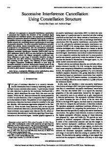
The initial RF transmitter positions are identified by taking the first maximum from Figure 12 and assigning it to the first transmitter location. Next the DOA estimates within +/-5 degrees of this transmitter are assigned to this particular transmitter and removed from the plot. After removing these lines, the highest peak is again located and assigned to the second RF transmitter.
The DOA estimation algorithm assumed the array to be horizontal, which was not always the case (e.g. when driving up hills) Some of the antenna positions were changed slightly after the calibration run. The data from the antenna array was time-stamped using the internal clock of a laptop computer, which may not have been completely stable. This could have resulted in a slight mismatch between the time of the DOA estimate and the antenna array position.
• •
The above procedure is repeated for each RF transmitter. The sequence of images obtained are shown in Figure 13. It was found that the actual grid size used in the analysis was important and should be matched to the estimated accuracy of the DOA estimates.
Next consider the problem of estimating the exact RF transmitter positions by triangulation. In the following analysis a least squares fit on the DOA estimates shown in Figure 10 was used to obtain the interference source locations. The least squares fit was carried out in a three stage process: • The approximate RF transmitter locations and number of transmitters were estimated. • The DOA estimates corresponding to each RF transmitter were grouped together. • A more precise estimate of each RF transmitter location was obtained by doing a least squares fit on the DOA estimates assigned to each transmitter.
Finally, a least squares fit was carried out on the DOA estimates assigned to each RF transmitter. The results of this least squares fit are shown in Figure 14. Note that the final step of applying the least squares fit did not improve the accuracy of the localisation all the time. 10
10
8
8
North6 (Km)
The first step in the above sequence (the initial estimation of RF transmitter locations) was carried out as follows: • Partition the map up into a grid of size 200m by 200m. • For each DOA estimate: increment the counter in those grid cells which line up with the DOA estimate
4
4
2
2
0
0
-2 -10 10
Applying the above procedure gives a colorscale map where the maxima correspond to the points where most of the DOA lines are intersecting, as shown in Figure 12.
-5
0
Nor th (K m)
-5
6
6
North 4 (Km)
4
2
2
0
0
-5
0
5
-2 -10
0 East (Km)
-5
0
East (Km)
Figure 13: Sucessive interference source localisation.
6
4
2
0
-2 -10
-2 -10 10
8
East (Km) 8
5
East (Km)
8
-2 -10
10
6
-5
0
5
East (Km)
Figure 12: DOA estimates mapped onto a regular grid of 200 m resolution.
ION GPS 2002, 24-27 September 2002, Portland, OR
618
10
A circular antenna array was used with a total of 8 antenna elements. The antenna spacing used in these trials was slightly larger than on most adaptive antenna arrays to improve the DOA estimation accuracy.
5 4
8
North (Km)
6
The accuracy of the DOA estimates from the antenna array were estimated to be within at least +/- 1.5 degree over calibration data, which was roughly equal to the accuracy of the ground truth DOA measurement. The DOA accuracy obtained in the actual localisation run was slightly worse and had a standard deviation of 3 degrees for the strongest source. This loss in accuracy may have been partly due to other error sources, such as errors in the estimated heading of the vehicle. The array can estimate the DOA of multiple signals at any one time, however in these trials only the two strongest signals were used at any time instant. The DOA accuracy of the second strongest signal was worse than the strongest signal and had a standard deviation of 14 degrees. Overall, it was found that the above DOA estimation accuracies were sufficient to localise multiple interference sources, to within approximately 100 to 300 metres.
3
4
2
1
0
-8
-6
2 -4
-2 East (Km)
0
2
4
Interference source location Initial estimate of interference source location
Least squares fit of interference source location
Future work could include the use of more advanced array calibration techniques to improve the accuracies of the DOA estimates. In particular, the GPS satellite signals could be used to self-calibrate the array. It may also be possible to use the GPS signals to accurately calculate the heading and attitude of the antenna array.
Van trajectory
Figure 14: Estimated interference source locations. The actual locations of the exact source locations are compared with those estimated from the least squares fit in Table 1. X Co-ordinate Y Co-ordinate Distance (Km) (Km) Error Source Exact Estimate Exact Estimate (Km) 1 -4.71 -4.40 0.40 0.32 0.32 2 2.09 1.91 0.22 0.34 0.22 3 3.19 3.07 3.90 3.90 0.10 4 3.32 3.31 9.05 9.05 0.08 5 -7.30 -7.32 8.91 8.91 0.03
REFERENCES M. Geyer, R. Frazier, “FAA GPS RFI Mitigation Program”, ION GPS’99, pp. 107-113. K. Gromov, D. Akos, S. Pullen, P. Enge, B. Parkinson, “GIDL: Generalized Interference Detection and Localization System”, ION GPS 2000, September 2000.
Table 1: Errors in RF transmitter location estimates.
K. Falcone, “Use of Anti-Jam Equipment in Location of Interference Sources”, ION GPS Sept. 2001
This paper has not considered the actual power levels of the interference sources or the sensitivity of the antenna array. This is partly because the power levels of the transmitters were changing during the course of the trial, and different transmitters were being switched on and off at different time periods. Further analysis of the data, and perhaps a more controlled experiment is required to experimentally quantify the DOA and hence localisation accuracy versus SNR.
K. Bond, J. Brading “Location of GPS Interference using Adaptive Antenna Technology”, ION GPS Sept. 2000. M. Trinkle, D. Gray, “Adaptive Antenna Arrays for GPS Interference Localisation”, SatNav 2001, July, 2001a. M. Trinkle, D. Gray, “GPS Interference Mitigation: Overview and Experimental Results”, SatNav 2001, July, 2001b.
CONCLUSION
C. Therrien, “Discrete Random Signals and Statistical Signal Processing”, Prentice Hall Signal Processing Series, 1992.
This trial has investigated the used of a mobile GPS adaptive antenna array to simultaneously reject and localise multiple RF transmitters operating in the GPS band. ION GPS 2002, 24-27 September 2002, Portland, OR
619