GPU-based Rendering of Sparse Low-degree IMplicit ... - CiteSeerX

GPU-based Rendering of Sparse Low-degree IMplicit Surfaces Takashi Kanai The University of Tokyo

Yutaka Ohtake Hiroaki Kawata Kiwamu Kase RIKEN, VCAD Modeling Team

Abstract Implicit surface is a well-known surface representation. Geometric details of an object can be represented using less surface primitives than other representations such as polygonal meshes. In this paper, we propose a fast and a direct rendering method of SLIM (Sparse Low-degree IMplicit) surfaces using recent programmable GPUs. Our approach establishes a direct rendering of implicit surfaces based on the ray casting approach. Geometric processes such as an intersection between a ray and an implicit surface and blending for PU (Partition of Unity) are performed in the fragment program on GPUs. For large models, a hierarchical structure of a SLIM surface can be used for LOD rendering or view frustum culling to speed up the rendering. We demonstrate that highly parallel processing using GPUs enables efficient rendering of implicit surfaces. CR Categories: I.3.5 [Computer Graphics]: Computational Geometry and Object Modeling—Curve, Surface, Solid and Object Representations; I.3.7 [Computer Graphics]: Three-Dimensional Graphics and Realism—Visible line/surface algorithms Keywords: Implicit surface, SLIM, Ray casting, GPU, Fragment program.

1

Introduction

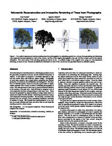
Figure 1: Left: the “moai” mesh (20K triangles) rendered by Phong shading. Right: A SLIM surface approximation of the mesh vertices (5K quadratic primitives) rendered by our GPU-based method. While almost the same geometrical details are approximated, the polygonal artifacts are eliminated.

Implicit surfaces including blobby model [Muraki 1991], metaballs [Nishimura et al. 1985], soft objects [Wyvill et al. 1986], and RBF (Radial-Basis Functions) [Savchenko et al. 1995; Carr et al. 2001] are well-known surface representations. The combination of multiple implicit surfaces can define a solid model strictly. From points with normal vectors, a volumetric field of an object can be defined by a set of implicit surfaces. In this field inside or outside of an object can be defined and the zero-set of such a volumetric field represents an iso-surface which approximates points. In these representations, a detailed smooth geometry of an object can be represented using less number of primitives than a polygonal mesh widely used in 3DCG applications.

On the other hand, a point on such an implicit surface cannot be represented explicitly. This poses as an inconvenience in rendering. There are roughly two approaches for displaying implicit surfaces. One is to create an intermediate polygon of a zero-set contour by using an iso-surface extraction method such as Marching Cubes [Lorensen and Cline 1987]. In this approach, however, both an isosurface polygon and a uniform or an adaptively subdivided volume grid has to be created, which requires additional memory and time. It is a disadvantage when deformed or animated implicit surfaces have to be especially rendered. In this case, iso-surface polygons have to be re-created for updating rendered images per frame.

MPU (Multi-level Partition of Unity) implicit surfaces [Ohtake et al. 2003] or SLIM (Sparse Low-degree IMplicit) surfaces [Ohtake et al. 2005] are recently-developed non-conforming implicit surface representations. In these surface representations, each node has a support sphere and a low-degree implicit polynomial function. A position or its derivative of a point on a surface is calculated by the weighted sum of a set of function values of several overlapped implicit surfaces. Since MPU or SLIM itself has a hierarchical tree structure, a set of implicit surfaces with arbitrary resolution can be quickly extracted.

The other approach is to render directly by ray tracing or ray casting. In this approach, a ray from an eye is defined for each pixel of an image and an intersection between such a ray and an iso-contour is computed. Since a per-pixel shading color is calculated by using an exact position and normal vector, a high quality image can be generated (see Figure 1). One disadvantage is that this type of method has a high per-pixel computational cost, which makes it difficult to achieve real-time rendering by using traditional computational resources such as CPUs. In this paper, a method to directly render SLIM surfaces using recent programmable GPUs (Graphics Processing Units) is proposed. Current GPUs have the ability as a processor for general-purpose scientific computation due to their high parallelism and flexibility. Our approach achieves fast and direct rendering of implicit surfaces by the per-pixel computation of positions and normal vectors in the programmable shader. In [Ohtake et al. 2005], they also propose a method to render SLIM surfaces directly by CPUs and orthogonal

projections in addition to the definition of SLIM surfaces. In contrast, our approach establishes fast rendering by using GPUs and can create more sophisticated rendering images by perspective projection.

2

Implicit function texture

Related Work

GPU

A number of ray-casting based rendering approaches for geometric models have been proposed in the past. This type of methods include the ray tracing for point-based models [Adamson and Alexa 2003; Wald and Seidel 2005; Adams et al. 2005; Tejada et al. 2006], the volume rendering [Engel et al. 2001; Westermann and Sevenich 2001; Kruger and Westermann 2003; Hadwiger et al. 2005], and the ray casting for implicit surfaces [Nishita and Nakamae 1994; de Groot and Wyvill 2005]. Specifically [Hadwiger et al. 2005] proposed a GPU-based ray casting algorithm for rendering volume data. However, this work is concerned with surfaces over a voxel grid, not surfaces described in implicit polynomials as like our method. There are several GPU-based approaches which are closely related to our approach. [Gumhold 2003] proposed a GPU-based ray casting method by computing ray-ellipsoid intersections for tensor field visualizations. More recently, [Sigg et al. 2006] extended his approach to handle perspective projections and applied to molecular rendering. [Loop and Blinn 2006] proposed a GPU-based algorithm for rendering up to fourth-order algebraic surfaces defined by trivariate B´ezier tetrahedra. All three approaches adopt a ray casting method for rendering implicit surfaces to achieve high quality rendering. The most significant difference compared to their approaches is that our approach determines contour iso-surfaces defined by several overlapping implicit polynomials in the programmable shaders of GPUs. This includes the blending operation for PU (Partition of Unity) evaluation discussed in Section 3.3.

3

Direct Rendering of SLIM Surfaces on GPUs

In this section we describe a direct rendering method of SLIM surfaces [Ohtake et al. 2005] by GPUs. A SLIM surface is defined as the hierarchical tree structure of nodes including support spheres. Here, we consider only the rendering for leaf nodes of such a tree structure. Let the radius and the center position of a support sphere in leaf nodes be ri , ci (i = 1, . . . , N, N is the number of leaf nodes). In the original definition of a SLIM surface [Ohtake et al. 2005], a node has more than one low-degree implicit polynomial up to cubic. For the convenience of explanation, each node has only a quadratic implicit polynomial fi (x) (x = (x, y, z)) consisting of ten coefficients: fi (x)

=

a0i x2 + a1i y2 + a2i z2 + a3i xy + a4i yz

+

a5i zx + a6i x + a7i y + a8i z + a9i = 0.

Rendering Billboards (or Point Sprite)

(1)

Our approach can however be easily extended to the case of higher degrees. We also assume that each implicit polynomial is defined on the relative coordinate system by setting a center point of a support sphere as the origin. Figure 2 illustrates the procedure of our rendering method. Our method is strongly motivated by the ray-casting based point rendering algorithm proposed in [Botsch et al. 2004] and [Botsch et al. 2005]. The core process of our algorithm consists of the following three passes executed in the programmable shader:

1st pass

2nd pass

Calculate an intersection point between a ray and an implicit function Z culling

Calculate an intersection point between a ray and an implicit function Compute gradients Blend points and gradients

Points ( p ) texture

Ωp

Points texture

3rd pass

Ωp

Division of points and gradients by the weight sum Shading

Gradients texture

Ωn

Display

Figure 2: Overview of our algorithm on GPUs.

1st pass: A ray from a viewpoint to a fragment is defined, and intersection points to an implicit polynomial f (x) = 0 are calculated. For such intersection points, the nearest point pˆ to a viewpoint is selected and is stored to a floating point texture Ωpˆ . 2nd pass: The same process of the first pass is performed to compute an intersection point p and its gradient ∇ f (p). They are blended and stored in the separate textures Ωp , Ωn . 3rd pass: A position and a normal vector of a surface are computed using p and ∇ f (p) respectively. Shading colors are computed using such values. As noted above, the same process (calculation of intersection points between a ray and an implicit polynomial) is applied in both the first and second passes. This is because we select points to be blended in the second pass using a point calculated in the first pass for a fragment (see details in Section 3.3). In the following subsections, we describe the detail of the algorithm.

Note. In the following subsections, we describe the functions and environment variables of OpenGL libraries in addition to the explanation of our algorithm for the convenience of the implementation. However, our algorithm can also be implemented using DirectX.

3.1

Drawing Supported Regions by Billboards

In the first and second passes, an intersection point between a ray and implicit polynomial is computed in the fragment program. Basically, a fragment needed for this computation can be created by drawing a support sphere surrounding an implicit polynomial and then by applying the rasterization of such a sphere.

w h

(0, 0)

c0

(3, 0)

a a a a a a a a a r0 a 0 0 2 0

1 0

3 0 5 0

4 0

6 0 8 0

7 0 9 0

c1

a10 a11 a13 a14 a16 a17 a15 a18 a19 r1 a12 R G B A

Figure 4: Storing implicit surface parameters to a two-dimensional floating point texture.

Figure 3: Rendering rectangular polygons by billboards. Left: “moai” model (5K nodes). Right: “david’s head” model (200K nodes).

However, drawing spheres themselves has high computational costs. To display such a sphere, an approximated polygon is generally used. Although a more subdivided polygon can achieve higher accuracy, the number of polygons to be displayed is exponentially increased. Instead of using a sphere approximated by polygons, we display the same region on the screen by a regular rectangle whose size is a radius of a sphere. The computational cost is dramatically reduced since only a rectangle is drawn for generating the same number of fragments on the screen as that of a sphere. In this case, we have to ensure that the same size of region is drawn when we display such a rectangle. To do so, a rectangle should always turn in front for arbitrary viewpoints. Two approaches can be considered to create such an “always-infront” rectangle. One is to use a billboard and the other is to utilize a point sprite (GL ARB point sprite) which is one of the recent functionalities on GPUs. In the case of using billboards, the positions of four vertices of a rectangular polygon are computed to turn in front in advance and they are transferred to a GPU. On the other hand, in the case of using point sprites, only the center position of a rectangular polygon (in our case the center ci of a support sphere) needs to be transferred to a GPU. The sprite size on the screen can be computed in the vertex program. Hence in the view of transferring positions to a GPU, the point sprite method should be a better choice compared to the use of billboards. One critical disadvantage in the use of point sprites is that the maximum sprite size on the screen is limited depending on GPU hardware1 . When an object is magnified to a certain extent, large holes appear. Our first choice here is then to use billboards. Figure 3 shows the display results of objects by billboards. In the point-based rendering approaches, the bounding box computation on screen space for perspectively-accurate rendering is required because their rendering primitives are ellipses [Zwicker et al. 2004]. In contrast, such perspective corrections are not needed in our scheme since we use only spheres as rendering primitives. 1 This

parameter can be investigated using an environment variable GL POINT SIZE MAX ARB. For example, a value measured on nVIDIA GeForce 7900 GTX is 63.375.

3.2

Preparing Implicit Surface Textures

In order to access parameters of implicit surfaces from fragment programs on GPUs in the first and second passes, these parameters are stored as two-dimensional floating point textures in advance. Fourteen floating points, a center position ci and a radius ri of a support sphere, coefficients of an implicit polynomial (a0i , a1i , . . ., a9i ), are stored for a node. Figure 4 illustrates our scheme for storing implicit surface parameters to a floating-point texture. Since four floating points can be stored in each RGBA pixel, four pixels are at least required to store fourteen floating points for each node of a SLIM surface. In our scheme, a center position ci and a radius of a support sphere ri are stored to the first pixel of the four. Coefficients of an implicit polynomial (a0i , a1i , . . ., a9i ) are then stored to the remaining three pixels. Note that other schemes to store such fourteen floating points to four pixels are also possible. Our scheme described here is only an example. To access a texture on the GPU, the first pixel coordinate (wi , hi ) of the corresponding four pixels is assigned to each node i. In billboard rendering, this pixel coordinate is set as a texture coordinate when setting four vertices of a rectangular polygon. A texture coordinate is inherited to a set of fragments via the rasterization, and is used to fetch a corresponding set of implicit surface parameters in the fragment program. Since the texture size for preparation is limited depending on GPU hardware2 , multiple textures have to be prepared when the number of nodes exceeds a limit size.

3.3

Computing Positions and Normal Vectors of Implicit Surfaces

Computing intersection points. Figure 5 illustrates the procedure to compute intersection points between a set of nodes (implicit surfaces) and a ray. This computation is done in the local coordinate system whose origin is the center point of a support sphere. Prior to the computation, a view position and a fragment are converted to such a local coordinate system respectively. Let a screen coordinate (NDC, Normalized Device Coordinate) of a fragment be fs . A formula to convert fs to a fragment f in a local coordinate system is as follows: f

=

(PM)−1 fs − ci ,

(2)

2 This parameter can be investigated using an environment variable GL MAX RECTANGLE TEXTURE SIZE EXT. Since a value measured on nVIDIA GeForce 7900 GTX is 4096, (4,096×4,096) / 4 = 4,194,304 nodes can be stored in a texture.

Implicit function p ~ Blended point p ~ and normal vector n Viewpoint e

Intersection point

Screen Fragment f

Support sphere

Figure 5: Illustration of computing intersection points between implicit surfaces and a ray. This point is selected.

Figure 7: Grayscale images of Z values. Left: Rendering result of billboards. Right: Result with applying Z corrections. value Z ′ by transforming an intersection point p is then: Z′ =

Implicit function Billboard

Figure 6: Issue of Z culling for billboard rendering. A point of an outline circle is incorrectly selected. where P, M denote the projection matrix and the model view matrix respectively, and ci denotes a center position of a support sphere. Using a view position at a local coordinate system e, a ray x = f + t (f − e) is defined. An intersection point between a ray and an implicit polynomial fi (x) at a node i: fi (f + t(f − e)) = 0,

(3)

is a quadratic equation over a parameter t and can be solved analytically. In case two points are computed, the nearest one to a view position is selected. We only consider intersection points in a support sphere. To do so, the distance from an intersection point to a center point and a radius are compared to select an active intersection point. ˆ Several intersection points may be 1st pass: Computing p. computed for a fragment because billboards projected to screen space are overlapped. In the first pass, the closest point to a view position pˆ (one of black-filled circles in the left of Figure 5) is selected. This can be done by Z buffer culling. pˆ is used to remove points farther from it (e.g. an outline circle in Figure 5) in the second pass. A computed pˆ is once stored to a floating point texture Ωpˆ as an output of a fragment program. A render-to-texture function by FBOs (Frame-Buffer Objects, GL EXT framebuffer object) is used here to reduce the bottleneck for the transmission of such outputs between a GPU and CPU. Z correction. In our approach, fragments are computed from billboards. A current Z value of a fragment then comes from the perspective projection of a billboard. However, a Z value of an intersection point between a ray and an implicit polynomial and that of a billboard is in general different. This leads to the failure of Z culling. Figure 6 illustrates this situation. In this case, an intersection point farther from a view point is selected due to its Z value. To resolve this issue, Z correction is performed by computing an exact Z value from the projection of an intersection point. A new Z

ps .z − Zn , Z f − Zn

ps = PMp,

(4)

where Zn , Z f denotes Z values of near and far planes in the view frustum respectively. ps .z denotes a z-coordinate of a position ps in screen space after the transformation of p. Z is then replaced to Z ′ in the fragment program of the first pass. Figure 7 shows the grayscale images of Z values for the comparison of with and without Z correction. White pixels show the small Z values. It can be seen in the left figure that jaggies appear due to the use of Z values for billboards. In contrast, smooth Z values are confirmed in the right figure by applying Z corrections.

Computing positions and normal vectors. In the second and third passes, a position p˜ and a normal vector n˜ (a red-filled circle with an arrow in Figure 5) of an implicit surface are computed for each fragment. In our approach, a point on a SLIM surface is evaluated as a PU (Partition of Unity) of neighbor points p j ( j = 1 . . . M, M is the number of neighbor points) to pˆ on a ray (called the ray-based PU [Ohtake et al. 2005]): p˜ =

∑M j ω jp j ∑M j ωj

,

(5)

where ω j denotes a weight defined as a Gaussian function. A normal vector is also evaluated as follows: n˜ =

n , |n|

n=

∑M j ω j ∇ f j (p j ) ∑M j ωj

,

(6)

where ∇ f j (p j ) denotes a gradient of an implicit surface f j at a point p j. An issue to be noted here is that division operations appearing in Equations (5) and (6) cannot be executed in a fragment program. Computations of positions and normal vectors are hence performed in the two separated passes as in [Botsch and Kobbelt 2003]. In the second pass, weighted sums of both numerators and denominators in Equations (5) and (6) are separately computed. Using such outputs, p˜ and n˜ are computed by only applying division operations in the third pass. 2nd pass: Blending intersection points. In the second pass, the same process of the first pass is applied to compute an intersection point p. Additionally, pˆ is fetched from Ωpˆ . A corresponding

pixel coordinate to obtain pˆ can be calculated from a screen coordinate of a fragment. pˆ is used to select the neighbor points from several overlapped intersection points p of a fragment. This is done by comparing the distance from pˆ to p with the radius of a support sphere ri . For the selected point p only, the gradient of an implicit polynomial ∇ f (p) is also computed. Both two weighted sums of those neighbor points and their graM M M dients (∑M j ω j p j , ∑ j ω j ), (∑ j ω j ∇ f j (p j ), ∑ j ω j ) are next computed and stored to floating point textures Ωp , Ωn separately. These computations are done by blending which is one of the functionalities of GPUs. To use the blending functionality, the depth test by Z buffer is first disabled and the blending (GL BLEND) is then enabled. Moreover, the blend function is set to “the weighted sum by an input alpha value”3 . M M M Finally, two outputs (∑M j ω j p j , ∑ j ω j ), (∑ j ω j ∇ f j (p j ), ∑ j ω j ) of a fragment program are set. These can be stored to textures separately by using multiple draw buffer (GL ARB draw buffers) which is one of the functionalities of recent GPUs.

˜ n˜ and shading. In the third pass, 3rd pass: Computing p, a rectangular polygon which has the same resolution as a frame buffer (or a floating point texture Ωp , Ωn ) is drawn. A pixel coordinate of a fragment can be then acquired by rasterization. Using M this pixel coordinate, a pair of four pixel values (∑M j ω j p j , ∑ j ω j ), M M (∑ j ω j ∇ f j (p j ), ∑ j ω j ) are fetched from floating point textures Ωp , Ωn respectively. A position p˜ and a normal vector n˜ of an implicit surface are now computed by dividing the first three elements of pixel values by a fourth element. Finally, a shading color ˜ n˜ to generate a final image. is computed using p,

3.4

LOD Rendering and View Frustum Culling

A SLIM surface has a hierarchical tree structure of nodes including implicit polynomials. Based on a tree structure, LOD (Level-OfDetail) rendering and view frustum culling can be performed efficiently using support spheres of nodes. In LOD rendering, child tree nodes are traversed from a root node. For a node, if the radius of a support sphere in screen space is less than a threshold (a few pixels here), its parent node is rendered. In view frustum culling, the basic process is the same. The only difference is that the inside/outside test of a node to a view frustum is performed instead. Figure 8 shows the comparison of resulting images between the rendering of only leaf nodes (left) and LOD rendering (right) of a “david” model. It can be seen that almost no visual difference appears while the number of nodes in LOD rendering is approximately one-ninth of that in the rendering of leaf nodes.

4

Results and Discussion

Figure 9 shows the rendering results of example models used in the measurement of computational time. In our approach, high quality rendering is achieved because fragment-based computations of positions and normal vectors are performed. Note that in our approach, the blending operation is executed on a 16-bit pixel buffer due to the limitation of GPU hardware. However, it can be said that such a limitation does not lead to any visual defects. 3 This

is done by setting glBlendFunc(GL SRC ALPHA, GL ONE).

Figure 8: Control of nodes in LOD rendering of “david” model. Left: leaf nodes (932,720 nodes). Right: LOD nodes (126,466 nodes).

Table 1 shows the statistical summary of measured computation times for the models described in this paper. In this table, the computational times measured on CPUs are from the software implemented in [Ohtake et al. 2005]. Note that [Ohtake et al. 2005] proposes a rendering method applying orthogonal projection for simplifying computation compared to our approach. It can be seen from the table that the computation time in our approach on GPUs is roughly three to seven times faster than the rendering by CPUs. The rendering speed is more effective especially for models with a small number of nodes. This is due to the effect of parallelization by GPUs. Since our approach is based on a ray casting method, the large number of fragments filling the screen yields considerably more computation time. This can be verified by comparing the results of “moai” and “dino”. The rendering time of “moai” is twice faster than that of “dino”, while the number of nodes in “moai” is less than that of “dino”. This is because the filled fragments of “moai” are much larger than those of “dino”. On the other hand, the speed up of rendering is not so much of a focus in our approach for large models, especially for “lucy” and “david”. In these models, the obstacle lies in the process to transfer nodes (billboards) from a CPU to a GPU. In this case, it is much more effective to reduce the nodes themselves to be transferred. In fact, it have been confirmed that the rendering speed is twice to three times faster using the LOD technique.

5

Conclusions and Future Work

In this paper, a fast rendering method for SLIM surfaces, which is a type of point-based implicit surface, has been proposed. Our

Figure 9: Rendering results of models used for the measurement of the computational time. From upper left: dino, armadillo, lucy. From bottom left: feline, xyzrgb dragon. A magnified view of lucy’s head is shown in a frame of right figure. model moai dino feline armadillo xyzrgb dragon lucy david

#total nodes 6,948 7,783 20,891 31,712 242,018 915,151 1,221,100

#leaf nodes 5,421 6,009 16,175 24,662 185,050 691,978 932,720

CPU (fps) 2.91 7.09 4.00 4.27 2.79 1.12 0.93

GPU (fps) 21.53 44.92 23.79 22.97 12.86 3.50 2.63

GPU (LOD) (fps) 6.45 7.08

#LOD nodes 130,696 126,466

Table 1: Statistical summary of computation times. From left to right: model name, number of all nodes, number of leaf nodes, computation time by CPUs (fps), computation time of leaf nodes by GPUs (fps), computation time of LOD nodes (fps), the number of LOD nodes. A window size is 512 × 512 for all tests. These are measured on a PC with Pentium D 840 (3.2GHz) CPU and nVIDIA GeForce 7900 GTX GPU. approach achieves high quality rendering by computing the position and normal vector for a fragment by implementing a ray-based PU. We have demonstrated that computation time is roughly three to seven times faster compared to CPU-based rendering, and roughly twice to three times faster for large models. Two future directions are mainly considered. One is an extension of our approach to address sharp features such as creases and corners. In SLIM surfaces, sharp features are treated by special processes including Boolean operations. We should consider how to implement such Boolean operations on GPUs. The other is the direct rendering of other implicit surface representations such as metaballs and blobby models. However, we think that these representations can be rendered by using our rendering framework on GPUs.

Cyberware Inc. (dino).

References A DAMS , B., K EISER , R., PAULY, M., G UIBAS , L. J., G ROSS , M., AND D UTR E´ , P. 2005. Efficient raytracing of deforming point-sampled surfaces. Computer Graphics Forum (Proc. Eurographics 2005) 24, 3, 677–684. A DAMSON , A., AND A LEXA , M. 2003. Ray tracing point set surfaces. In Proc. Shape Modeling International 2003, IEEE CS Press, Los Alamitos CA, 272–282.

Acknowledgements

B OTSCH , M., AND KOBBELT, L. P. 2003. High-quality pointbased rendering on modern GPUs. In Proc. 11th Pacific Conference on Computer Graphics and Applications, 335–343.

The models used in this paper are courtesy of California Institute of Technology (feline), the Stanford 3D Scanning Repository (armadillo, xyzrgb dragon, lucy, david), Aizu University (moai), and

B OTSCH , M., S PERNAT, M., AND KOBBELT, L. P. 2004. Phong splatting. In Proc. Symposium on Point-Based Graphics 2004, Eurographics Association, 25–32.

B OTSCH , M., H ORNUNG , A., Z WICKER , M., AND KOBBELT, L. 2005. High-quality surface splatting on today’s GPUs. In Proc. 2nd Eurographics Symposium on Point-Based Graphics, Eurographics Association, Aire-la-Ville, Switzerland, 17–24.

S IGG , C., W EYRICH , T., B OTSCH , M., AND G ROSS , M. 2006. GPU-based ray-casting of quadratic surfaces. In Proc. 3rd Eurographics Symposium on Point-Based Graphics, Eurographics Association, Aire-la-Ville, Switzerland, 59–65.

C ARR , J. C., B EATSON , R. K., C HERRIE , J. B., M ITCHELL , T. J., F RIGHT, W. R., M C C ALLUM , B. C., AND E VANS , T. R. 2001. Reconstruction and representation of 3D objects with radial basis functions. In Computer Graphics (Proc. SIGGRAPH 2001), ACM Press, New York, 67–76.

T EJADA , E., G OIS , J. P., N ONATO , L. G., C ASTELO , A., AND E RTL , T. 2006. Hardware-accelerated extraction and rendering of point set surfaces. In Proc. Eurographics / IEEE VGTC Symposium on Visualization, Eurographics Association, Aire-laVille, Switzerland, 21–28.

G ROOT, E., AND W YVILL , B. 2005. Rayskip: Faster ray tracing of implicit surface animations. In Proc. 3rd International Conference on Computer Graphics and Interactive Techniques in Australasia and South East Asia (GRAPHITE ’05), ACM Press, New York, 31–36.

WALD , I., AND S EIDEL , H.-P. 2005. Interactive ray tracing of point-based models. In Proc. 2nd Eurographics Symposium on Point-Based Graphics, Eurographics Association, Aire-la-Ville, Switzerland, 1–8.

DE

E NGEL , K., K RAUS , M., AND E RTL , T. 2001. High-quality preintegrated volume rendering using hardware-accelerated pixel shading. In Proc. ACM SIGGRAPH / EUROGRAPHICS Workshop on Graphics Hardware, ACM Press, New York, 9–16. G UMHOLD , S. 2003. Splatting illuminated ellipsoids with depth correction. In Proc. Vision, Modeling, and Visualization Conference (VMV), 245–252. ¨ H ADWIGER , M., S IGG , C., S CHARSACH , H., B UHLER , K., AND G ROSS , M. 2005. Real-time ray-casting and advanced shading of discrete isosurfaces. Computer Graphics Forum (Proc. Eurographics 2005) 24, 3, 303–312. K RUGER , J., AND W ESTERMANN , R. 2003. Acceleration techniques for GPU-based volume rendering. In Proc. IEEE Visualization 2003, IEEE CS Press, Los Alamitos CA, 287–292. L OOP, C., AND B LINN , J. 2006. Real-time GPU rendering of piecewise algebraic surfaces. ACM Transactions on Graphics (Proc. SIGGRAPH 2006) 25, 3, 664–670. L ORENSEN , W. E., AND C LINE , H. E. 1987. Marching cubes: A high resolution 3D surface construction algorithm. In Computer Graphics (Proc. SIGGRAPH ’87), ACM Press, New York, 163– 169. M URAKI , S. 1991. Volumetric shape description of range data using blobby model. In Computer Graphics (Proc. SIGGRAPH ’91), ACM Press, New York, 227–235. N ISHIMURA , H., H IRAI , M., K AWAI , T., K AWATA , T., S HI RAKAWA , I., AND O MURA , K. 1985. Object modeling by distribution function and a method of image generation. Trans. IEICE J68-D, 4, 718–725. (in Japanese). N ISHITA , T., AND NAKAMAE , E. 1994. A method for displaying metaballs by using bezier clipping. Computer Graphics Forum (Proc. Eurographics ’94) 13, 3, 271–280. O HTAKE , Y., B ELYAEV, A. G., A LEXA , M., T URK , G., AND S EI DEL , H.-P. 2003. Multi-level partition of unity implicits. ACM Transactions on Graphics (Proc. SIGGRAPH 2003) 22, 3, 463– 470. O HTAKE , Y., B ELYAEV, A. G., AND A LEXA , M. 2005. Sparse low-degree implicits with applications to high quality rendering, feature extraction, and smoothing. In Proc. 3rd Eurographics Symposium on Geometry Processing, Eurographics Association, Aire-la-Ville, Switzerland, 149–158. S AVCHENKO , V. V., PASKO , A. A., O KUNEV, O. G., AND K U NII , T. L. 1995. Function representation of solids reconstructed from scattered surface points and contours. Computer Graphics Forum 14, 4, 181–188.

W ESTERMANN , R., AND S EVENICH , B. 2001. Accelerated volume ray-casting using texture mapping. In Proc. IEEE Visualization 2001, IEEE CS Press, Los Alamitos CA, 271–278. W YVILL , G., M C P HEETERS , C., AND W YVILL , B. 1986. Data structure for soft objects. The Visual Computer 2, 4, 227–234. Z WICKER , M., R ASANEN , J., B OTSCH , M., DACHSBACHER , C., AND PAULY, M. 2004. Perspective accurate splatting. In Proc. Graphics Interface 2004, Morgan Kaufmann Publishers, San Francisco, CA, 247–254.