GPU Fast and Robust Computation for Barycentric Coordinates and

GPU Fast and Robust Computation for Barycentric Coordinates and Intersection of Planes Using Projective Representation Vaclav Skala Department of Computer Science and Engineering University of West Bohemia Plzen, Czech Republic http://www.VaclavSkala.eu Abstract—This paper describes algorithms for fast and robust GPU computation of barycentric coordinates and intersection of two planes. The presented algorithms are based on matrixvector operations which make the algorithms convenient for GPU or SSE based architectures. Also a new formula for finding the closest point of two planes intersection to the given point is given.

II.

PROBLEM FORMULATION

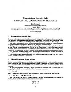
Intersection of two planes is a seemingly simple problem, see Fig.1.

Keywords-GPU, barycentric coordinates, two planes intersection, Plücker coordinates, closest point, homogeneous coordinates, projective space

I.

INTRODUCTION

Intersection of two planes is frequently used in geometric computations, e.g. in set operations with geometric objects given by triangular meshes. In spite of the simplicity of the problem, the standard formulas for computations are not robust in cases when given planes are almost parallel or parallel. Also barycentric coordinates computation, which leads to a solution of linear equations, is very often used to solve geometrical problems. In this paper standard approaches will be presented together with a new more robust approach especially convenient for GPU or SSE application based on projective representation. In the case of two triangles intersection computation, the vertices of triangles can be given in homogeneous coordinates and intersection of triangles can be computed directly without need to convert vertices coordinates to the Euclidean coordinates. This saves 18 division operations per one pair of triangles intersection computation, which leads to significant speed-up. Similarly, barycentric coordinates can be computed directly in the projective space if coordinates of vertices are in homogenous coordinates and the conversion to the Euclidean space is not needed, i.e. we save division operations as well. In the following the notation will be used:  for coordinates or vectors in  or homogeneous coordinates in the projective space  is the outer (cross) vector product  for dot (scalar) product

Figure 1: Intersection of two planes Let us assume two planes and vectors and

, Fig.1, given by two as: (1)

and (2) where: and We need to determine a line which is given as an intersection of those two planes if planes are “not parallel”. However due to the numerical precision in the floating point representation, the condition must be weaken to “not close to parallel”. There is the key problem, i.e. what does actually this condition mean and how it is defined from the algorithmic point of view. It can be seen that the line in the parametric form can be then determined as: (3) As the computation of the vector is simple and relatively precise, the “problem” is how to determine the point complying (1) and (2), reliably from the numerical

precision point of view. Unfortunately in some applications it can be found incorrect or non-robust solutions. III.

STANDARD SOLUTION

Standard formula for a line given as an intersection of two planes in the Euclidean space is given as: Then the “starting” point

is given as

(4)

Geometric transformations with points are described generally as: (6) where is a matrix in the case, or in the case. The advantage of the projective representation is that fundamental transformations like translation, rotation, scaling, shearing and projections are represented by a cumulative transformation matrix multiplied by a vector containing point’s coordinates. However, geometric transformations with lines in or planes in are given as: (7) as normal vectors are actually bivectors. It can be seen that the transformation matrices for lines or planes are different from the transformation matrix of points defining the given goe. V.

This formula is quite “horrible” one and for users is too complex to remember and they do not see from the formula comes from. It can be seen that coordinates are computed using division operation and division by is required. There is a legitimate question about specification of cases when division by causes floating point overflow or underflow. In many cases the programmer uses a sequence: ; if then Error but it can happen that the expression is , e.g. for the -coordinate, and the expression is actually “well conditioned”. The formula for computation is not convenient for GPU, nor SSE application, too. IV.

PROJECTIVE SPACE REPRESENTATION

The projective extension of the Euclidean space is often used in geometry, sometimes is “hidden” in the known formulas. Let us consider a point and its equivalent in the projective space . The mutual conversion is then given as [1],[3]: (5) It can be seen that it is actually one parametric set, i.e. a line passing the origin in the coordinate system, but origin is excluded. The extension to the case is straightforward. Homogeneous coordinates and the projective space representation is widely used in computer graphics to represent geometric transformations, projection operation etc.

PRINCIPLE OF DUALITY

The principle of duality in states that any theorem remains true when we interchange the words “point” and “line”, “lie on” and “pass through”, “join” and “intersection”, “collinear” and “concurrent” and so on. In the case of dual identities are “point” and “plane” etc. Once the theorem has been established, the dual theorem is obtained as described above [2], [5]. In other words, the principle of duality says that in all theorems in it is possible to substitute the term “point” by the term “line” and the term “line” by the term “point” and the given theorem stays valid. In the case of dual terms are “point” and “plane”. This helps a lot to solve some geometrical problems. A nice example of projective space representation and principle of duality application in the case is computation of a line given by two given points , Eq.(8) (8) and an intersection point

of two lines

, Eq.(9) (9)

It can be shown that computation of an intersection of two lines in E2 is dual to computation of a line given by two points (it is actually a join operation). It means that there should be the same programming sequence for solving both dual cases [7], i.e.

(10)

and

VI. (11)

In the case of E3 a plane given as a join of three points and dual problem, i.e. an intersection of three planes, can be computed as [8]:

PLÜCKER COORDINATES

The Plücker coordinates are often used in robotics and geometrical problems solutions, e.g. in a ray-triangle intersection detection and intersection computation [4]. Let us consider two points in the homogeneous coordinates: (14) definining a line . The Plücker coordinates anti-symmetric matrix are defined as:

(15)

(12)

Let us define two vectors

and

of the

and

as: (16)

(13)

There are significant advantages of this approach:  Natural support for GPU computation leading to significant speed up.  There is no division operation used that is needed if an intersection is computed in the Euclidean space, like  

, which leads to instability in principle. There are no special cases which a programmer has to take care of, i.e. detection of collinearity etc. If points are given in homogeneous coordinates, transformation to the Euclidean coordinates is not required. It means that 6, resp. 9 division operations are not needed in the case of , resp. , and higher precision can be expected as well.

As a direct consequence it can be proved [9] that a solution of a linear system of equations is equivalent to an extended cross-product [9]. This is a significant result as instead of solving a linear system of equations we can use extended cross-product. It should be noted that replacing a solution of linear system of equations by the extended cross-product enables also further formal manipulation using linear algebra. As a typical example of this approach is computation of barycentric coordinates which can be used also for the case, when points are given in homogeneous coordinates.

It means that represents the “directional vector”, while represents the “positional vector”. It can be seen that for the Euclidean space ( ) we get: (17) where: are coordinates of points in the Euclidean space. The line given by two points in the homogeneous coordinates is then given as: (18) where are coordinates of points on the line . Due to the principle of duality in we can exchange “point” and “plane” in the Eq.(14). As the panes are given as: (19) Now, the matrix

is defined as (20)

and the rest is the same. However, an intersection of two planes is the case also often solved in computer graphics and vision. Unfortunately in many cases available solutions are not robust or formulas used are neither simple, like above, nor convenient for GPU use. This approach also requires normalization of the vector and division operations. In the following a new formulation of two plane intersection is presented and as the projective space is used for formulation and the solution is quite simple.

VII. INTERSECTION OF TWO PLANES Let us consider again two planes given in implicit form, i.e. , and given points in homogeneous coordinates, see Fig.1. (21) The directional vector of the line given as an intersection of those two planes is again given as: (22) An angle

between two planes

and

is given as: (23)

If the “standard” formula is used, the value is to be used for detection of close to singular cases or: (24) as this eliminates function computation in the vector normalization as well. Now, let us assume a plane passing the origin of the coordinate system having as a normal vector the vector , see Fig.1. Therefore the point is an intersection of three planes , and can be computed as a direct application of the principle duality in the case as a straightforward application of the Eq.(8) and Eq.(9):

Derivation of this formula is simple, fast and it is well suited for the GPU or SSE application as the cross product is an GPU instruction, see Appedix A VIII. BARYCENTRIC COORDINATES Barycentric coordinates are often used in many applications, not only in geometry. Barycentric coordinates computation leads to a solution of a system of linear equations. However it can be shown, that a solution of a linear system equations is equivalent to a cross product [7], [8], [10]. Therefore it is possible to compute barycentric coordinates using cross product for GPU oriented applications. Let us consider the case, i.e. interpolation between two points, and vector: (27) Then the projective barycentric coordinates are given as: (28) The Euclidean barycentric coordinates are given as: (29) Let us consider the case, i.e. interpolation between three points of the given triangle, and vectors: (30) The projective barycentric coordinates are given as: (31)

(25)

The Euclidean barycentric coordinates are given as: (32)

From the Eq.(25) we can write for the homogeneous coordinates

point using :

Let us consider the case, i.e. interpolation between four points of the given tetrahedron, and vectors: (33) Then projective barycentric coordinates are given as:

(26)

(34) The Euclidean barycentric coordinates are given as: (35)

The point is the closest point on the line to the origin of the coordinate system. As the computation is made in the projective space no division operation is needed. The actual decision on “singularity” of computation is postponed. As a determinant is multilinear, it is clear that normalization of plane’s equations to not needed. and it is not a way how to increase stability of computations. Even more we are getting a formula, which can be used for symbolic manipulation and computation as well.

How simple and elegant solution! It can be seen that the presented computation of barycentric coordinates is simple, convenient for GPU or SSE application. Even more, as we have assumed from the very beginning, there is no need to convert coordinates of points from the homogeneous coordinates to the Euclidean coordinates. As a direct consequence of that is that we save lot of division operations and also increase robustness of the computation.

IX.

THE CLOSEST POINT TO AN INTERSECTION OF PLANES

Finding the closest point on the intersection of two planes to the given point is not an easy problem. The usual solution is based on application of the Lagrange multipliers [6] leading to a solution of a system of linear equations with a matrix . This solution is computationally costly and not convenient for the GPU applications. Using projective representation we can easily solve the problem as follows. Let us assume given two planes: (36) with normal vectors: (37) Directional vector of a line given as an intersection of two planes and is determined as (38) and the “starting” point is determined as recently stated (39) and the plane is passing the origin with a normal vector , i.e. the plane is defined by . The solution is now quite simple applying the following steps:  Translate planes and so the given point is in the origin, transformation matrix is  Compute intersection of two planes, i.e. determine the directional vector of the line and the point  Translate the computed point using

XII. REFERENCES [1]

Bloomenthal,J., Rokne,J.: Homogeneous Coordinates, The Visual Computer, Vol.11,No.1, pp.15-26, 1994. [2] Coxeter,H.S.M.: Introduction to Geometry, John Wiley, 1969. [3] Hartley,R, Zisserman,A.: MultiView Geometry in Computer Vision, Cambridge Univ. Press, 2000. [4] Jimenez,J.J., Segura,R.J., Feito,F.R.: Efficient Collision Detection between 2D Polygons, Journal of WSCG, Vol.12, No.1-3, 2003 [5] Johnson,M.: Proof by Duality: or the Discovery of “New” Theorems, Mathematics Today, December 1996. [6] Krumm,J.: Intersection of Two Planes, Microsoft Research, Research note, 2000 [7] Skala,V.: A New Approach to Line and Line Segment Clipping in Homogeneous Coordinates, The Visual Computer, Vol.21, No.11, pp.905 914, Springer Verlag, 2005 [8] Skala,V.: Length, Area and Volume Computation in Homogeneous Coordinates, International Journal of Image and Graphics, Vol.6., No.4, pp.625-639, 2006 [9] Skala,V.: Barycentric Coordinates Computation in Homogeneous Coordinates, Computers & Graphics, Elsevier, ISSN 0097-8493, Vol. 32, No.1, pp.120-127, 2008 [10] Skala,V.: Projective Geometry, Duality and Precision of Computation in Computer Graphics, Visualization and Games, Tutorial Eurographics 2013, Girona, 2013 [11] Skala,V.: Projective Geometry and Duality for Graphics, Games and Visualization - Course SIGGRAPH Asia 2012, Singapore, ISBN 978-1-4503-1757-3, 2012

APPENDIX The cross product in 4D is defined as

The point is the closest point of the line to the given point . Even more, the parameter value to this point is . and can be implemented in Cg/HLSL on a GPU as follows: Again – an elegant solution, simple formula supporting matrix-vector architectures like GPU and parallel processing. X.

CONCLUSION

In this paper we have presented a new robust approach for a solution of selected geometrical problems using projective representation. This approach offers much simpler formulation, algorithms based on matrix-vector multiplications. Resulting formulas are convenient for GPU and SSE applications with achievable significant speedup as well. XI.

ACKNOWLEDGMENT

The author thanks to anonymous reviewers for their critical comments and hints that improved this paper significantly. Thanks also belong to students and colleagues at the University of West Bohemia, Plzen for their suggestions. The project was supported by the Ministry of Education of the Czech Republic, projects No.LG13047 and LH12181.

float4 cross_4D(float4 x1, float4 x2, float4 x3) { float4 a; a.x = dot(x1.yzw, cross(x2.yzw, x3.yzw)); a.y = - dot(x1.xzw, cross(x2.xzw, x3.xzw)); a.z = dot(x1.xyw, cross(x2.xyw, x3.xyw)); a.w = - dot(x1.xyz, cross(x2.xyz, x3.xyz)); return a; } or more compactly as float4 cross_4D(float4 x1, float4 x2, float4 x3) { return ( dot(x1.yzw, cross(x2.yzw, x3.yzw)), - dot(x1.xzw, cross(x2.xzw, x3.xzw)), dot(x1.xyw, cross(x2.xyw, x3.xyw)), - dot(x1.xyz, cross(x2.xyz, x3.xyz)) ); }