GPU implementation of a Helmholtz Krylov solver preconditioned by a ...

Journal of Computational and Applied Mathematics 236 (2011) 281–293

Contents lists available at SciVerse ScienceDirect

Journal of Computational and Applied Mathematics journal homepage: www.elsevier.com/locate/cam

GPU implementation of a Helmholtz Krylov solver preconditioned by a shifted Laplace multigrid method H. Knibbe ∗ , C.W. Oosterlee, C. Vuik Faculty of Electrical Engineering, Mathematics and Computer Science, Delft Institute of Applied Mathematics, Delft University of Technology, Mekelweg 4, 2628 CD Delft, The Netherlands

article

info

Keywords: GPU Helmholtz equation Krylov solvers Shifted Laplace multigrid preconditioner

abstract A Helmholtz equation in two dimensions discretized by a second order finite difference scheme is considered. Krylov methods such as Bi-CGSTAB and IDR(s) have been chosen as solvers. Since the convergence of the Krylov solvers deteriorates with increasing wave number, a shifted Laplace multigrid preconditioner is used to improve the convergence. The implementation of the preconditioned solver on CPU (Central Processing Unit) is compared to an implementation on GPU (Graphics Processing Units or graphics card) using CUDA (Compute Unified Device Architecture). The results show that preconditioned Bi-CGSTAB on GPU as well as preconditioned IDR(s) on GPU is about 30 times faster than on CPU for the same stopping criterion. © 2011 Elsevier B.V. All rights reserved.

1. Introduction Initially driven by the gamer market, GPUs (Graphics Processing Units) recently became suitable for high performance computing applications. A GPU or simply a graphics card is a multi-threaded, many-core processor which was originally developed for graphics processing. With the evolution of General Purpose computing on Graphics Processing Units (GPGPU) it became possible to accelerate a wide range of applications traditionally computed on a CPU (Central Processing Unit). One of the market leaders, Nvidia, developed a parallel computer architecture called CUDA (Compute Unified Device Architecture); see [1]. CUDA is a subset of the C language with some extensions which allows us to program the Nvidia GPUs in an easy way. The more recent initiative of Apple within Khronos Group is called OpenCL (Open Computing Language), that is an open standard and can be used to program CPUs, GPUs and other devices from different vendors. It has been shown that converting a CUDA program to an OpenCL program involves minimal modifications; see [2]. According to Du et al. [3], at this moment CUDA is more efficient on the GPU than OpenCL. In this paper we focus on iterative solvers for the Helmholtz equation in two dimensions on GPU using CUDA. The Helmholtz equation represents the time-harmonic wave propagation in the frequency domain and has applications in many fields of science and technology, e.g. in aeronautics, marine technology, geophysics, and optical problems. In particular we consider the Helmholtz equation discretized by a second order finite difference scheme. The size of the discretization grid depends on the wave number, that means, the higher the wave number the more grid points are required. For instance to get accurate results with 7-point discretization scheme in three dimensions, at least 10 grid points per wave length have to be used; see [4]. For high wave numbers the discretization results in a very large sparse system of linear equations which cannot be solved with direct methods on current computers within reasonable time. The linear system is symmetric but indefinite, non-Hermitian and ill-conditioned which brings difficulties when solving with basic iterative methods. The convergence of

∗

Corresponding author. E-mail addresses: [email protected] (H. Knibbe), [email protected] (C.W. Oosterlee), [email protected] (C. Vuik).

0377-0427/$ – see front matter © 2011 Elsevier B.V. All rights reserved. doi:10.1016/j.cam.2011.07.021

282

H. Knibbe et al. / Journal of Computational and Applied Mathematics 236 (2011) 281–293

the Krylov methods deteriorates with increasing wave number, so the need for preconditioning becomes obvious. In this paper we consider Bi-CGSTAB (see [5]) and IDR(s) (see [6]) as Krylov solvers. There have been many attempts to find a suitable preconditioner for the Helmholtz equation, see, for example, [7,8]. Recently the class of shifted Laplace preconditioners evolved, see [9–12]. In this work, we focus on a shifted Laplace multigrid preconditioner introduced in [11,13], to improve the convergence of the Krylov methods. The purpose of this work is to compare the implementations of the Krylov solver preconditioned by the shifted Laplace multigrid method in two dimensions on a CPU and a GPU. The interest is triggered by the fact that some applications on GPU are 50–200 times faster compared with a CPU implementation (see e.g. [14,15]). However there are no recordings of a Helmholtz solver on a GPU which we present in this paper. There are two main issues: the first one is the efficient implementation of the solver on GPU and the second one is the behavior of the numerical methods in single precision. Nevertheless, even on a modern graphics card with double precision units (for example, Tesla 20 series or Fermi), single precision calculations are still at least two times faster. The first issue can be resolved by knowing the insides of a GPU and CUDA. The second issue can be addressed by using mixed precision algorithms; see e.g. [16]. The paper is organized as follows. In Section 2 we describe the Helmholtz equation and its discretization. Also the components of the solver are described, including Krylov methods such as Bi-CGSTAB and IDR(s) and the shifted Laplace multigrid method. The specific aspects of the GPU implementation for each method are considered in detail in Section 3 and optimizations for the GPU are suggested. In Section 4 two model problems are defined: with constant and variable wave numbers. We solve those problems with Krylov methods preconditioned by the shifted Laplacian on a single CPU and a single GPU and compare the performance. Finally Section 5 contains conclusions and an outlook of this paper. 2. Problem description The two dimensional Helmholtz equation for a wave problem in a heterogeneous medium is considered

∂ 2 φ(x, y) ∂ 2 φ(x, y) − − (1 − α i)k2 (x, y)φ(x, y) = g (x, y), x, y ∈ Ω (1) ∂ x2 ∂ y2 where φ(x, y) is the wave pressure field, k is the wavenumber, α is the damping coefficient, g (x, y) is the source term. The −

corresponding differential operator has the following form:

A = −∆ − (1 − α i)k2 , where ∆ denotes the Laplace operator. In this paper we consider a rectangular domain Ω = [0, X ]×[0, Y ]. There are several boundary conditions:

• Dirichlet boundary conditions φ|∂ Ω = 0, • Non-reflecting boundary conditions – First order radiation boundary condition (described in e.g. [17,18])



 ∂ − ik φ = 0, − ∂η

(2)

where η is the outward unit normal component to the boundary. The disadvantage of this boundary condition is that it is not accurate for inclined outgoing waves. – Second order radiation boundary condition (described in [18]) 3

B φ|edge := − k2 φ − ik 2

B φ|corner := −2ikφ +

  2 − ∂φ 1 ∂ 2φ ± − = 0, ∂ xj 2 ∂ xi j=1,j̸=i

 2  − ∂φ = 0, ± ∂ xi i=1

(3)

(4)

where xi is a coordinate parallel to the edge for B φ|edge . The ± sign is determined such that for outgoing waves the non-reflecting conditions are satisfied. In many real world applications the physical domain is unbounded, and artificial reflections should be avoided. Therefore, we consider here the first order radiation boundary condition (2). 2.1. Discretization The domain Ω is discretized by an equidistant grid Ωh with the grid size h

Ωh := {(ih, jh) | i, j = 1, . . . , N }. For simplicity we set the same grid sizes in x- and y-directions. After discretization of Eq. (1) on Ωh using central finite differences we get the following linear system of equations: Aφ = g ,

A ∈ CN ×N , φ, g ∈ CN .

(5)

H. Knibbe et al. / Journal of Computational and Applied Mathematics 236 (2011) 281–293

283

The matrix A is based on the following stencil for inner points x ∈ Ωh /∂ Ωh :

 Ah =

1 h2

−1 4 − (kh)2 (1 − α i) −1

−1

 −1 .

(6)

The Dirichlet boundary conditions do not change the matrix elements at boundaries and the matrix will be structured and sparse. The first order radiation boundary condition (2) is discretized using a one-sided scheme, for example on the right boundary at xN +1 the solution can be expressed as uN +1,j =

uN , j 1 + ikhx

.

The matrix stencil at the boundaries change accordingly. 2.2. Solvers The discretized matrix A in (5) is complex-valued, symmetric, non-Hermitian, i.e. A∗ ̸= A. Moreover, for sufficiently large wave numbers k, the matrix A is indefinite, that means there are eigenvalues of A with a positive real part and eigenvalues with a negative real part. Furthermore, the matrix A is ill-conditioned. The mentioned properties of the matrix are the reason that the classical iterative methods (such as Jacobi et al., etc.) simply diverge. However, we may still be able to use them e.g. as smoothers for a multigrid method. 2.3. Krylov methods 2.3.1. Bi-CGSTAB One of the candidates to solve the discretized Helmholtz equation (5) is the Bi-CGSTAB method (see [5,19]). The advantage of this method is that it is easily parallelizable. However, even if the Bi-CGSTAB method converges for small wave numbers k, the convergence is too slow and it strongly depends on the grid size; see [4]. The original system of linear equations (5) can be replaced by an equivalent preconditioned system: AM −1 u = g ,

M −1 u = φ,

(7) −1

where the inverse of M is easy to compute. The matrix AM is well-conditioned, so that the convergence of Bi-CGSTAB (and any other Krylov method) is improved. As the preconditioner for Bi-CGSTAB we consider the shifted Laplace preconditioner introduced by Erlangga et al., see [11,13,12], which is based on the following operator:

M(β1 ,β2 ) = −∆ − (β1 − iβ2 )k2 ,

β1 , β2 ∈ R,

(8)

with the same boundary conditions as A. The system (5) is then preconditioned by M(β1 ,β2 ) = −L − (β1 − iβ2 )k2 I ,

β1 , β2 ∈ R

(9)

where L is the discretized Laplace operator, I is the identity matrix and β1 , β2 can be chosen optimally. Depending on β1 and β2 , the spectral properties of the matrix AM −1 change. In [12] the Fourier analysis shows that (9) with β1 = 1 and 0.4 ≤ β2 ≤ 1 gives rise to favorable properties that give rise to considerably improved convergence of Krylov methods (e.g. Bi-CGSTAB); see also [20]. 2.3.2. IDR(s) An alternative to Bi-CGSTAB to solve large non-symmetric linear systems of Eqs. (5) is the IDR(s) method, which was recently proposed in [6]. IDR(s) belongs to the family of Krylov methods and it is based on the Induced Dimension Reduction (IDR) method introduced by Sonneveld; see e.g. [21]. IDR(s) is a memory-efficient method to solve large non-symmetric systems of linear equations. We are currently using the IDR(s) variant described in [22]. This method imposes a bi-orthogonalization condition on the iteration vectors, which results in a method with fewer vector operations than the original IDR(s) algorithm. It has been shown in [22] that this IDR(s) and the original IDR(s) yield the same residual in exact arithmetics. However the intermediate results and numerical properties are different. The IDR(s) with bi-orthogonalization converges slightly faster than the original IDR(s). Another advantage of the IDR(s) algorithm with bi-orthogonalization is that it is more accurate than the original IDR(s) for large values of s. For s = 1 the IDR(1) will be equivalent to Bi-CGSTAB. Usually s is chosen smaller than 10. In our experiments we set s = 4, since this choice is a good compromise between storage and performance; see [23].

284

H. Knibbe et al. / Journal of Computational and Applied Mathematics 236 (2011) 281–293

The preconditioned IDR(s) method can be found in [22] and is given in Algorithm 1. Require: A ∈ CN ×N ; x, b ∈ CN ; Q ∈ CN ×s ; ϵ ∈ (0, 1); Ensure : xn such that ‖b − Axn ‖ ≤ ϵ Calculate r = b − Ax ; gi = ui = 0, i = 1, . . . , s; M = I ; ω = 1 ; while ‖r ‖ > ϵ do f = Q H r, f = (φ1 , . . . , φs ) ; for k=1:s do Solve c from Mc = f, c = (γ1 , . . . , γs )T ; ∑s v = r − i=k γi gi ; v = P −1 v ; ∑s uk = ωv + i=k γi ui ; gk = Auk ; for i=1:k-1 do qH g

α = µi i,ik ; gk = gk − α gi ; uk = uk − α ui ; end

µi,k = qHi gk , i = k, . . . , s, Mi,k = µi,k ; β = µφkk,k ; r = r − β gk ; x = x + β uk ; if k + 1 ≤ s then φi = 0, i = 1, . . . , k ; φi = φi − βµi,k , i = k + 1, . . . , s ; f = (φ1 , . . . , φs )T ; end end v = P −1 r ; t = Av ; ω = (tH r)/(tH t) ; r = r − ωt ; x = x + ωv ; end Algorithm 1: Preconditioned IDR(s) 2.4. Shifted Laplace multigrid preconditioner If Aφ = g in (5) is solved using the standard multigrid method, then conditions on the smoother and the coarse grid correction must be met. For the smoother the conditions are:

• k2 must be smaller than the smallest eigenvalue of the Laplacian; • The coarsest level must be fine enough to keep the representation of the smooth vectors. Furthermore, the standard multigrid method may not converge in case k2 is close to an eigenvalue of M. This issue can be resolved by using subspace correction techniques (see [24]). Because of the above reasons, we choose a complex-valued generalization of the matrix-dependent multigrid method in [25] as a preconditioner, as shown in (7). It provides an h-independent convergence factor in the preconditioner, as shown in [12]. In the coarse grid correction phase, the Galerkin method is used in order to get coarse grid matrices: MH = RMh P ,

(10)

where MH and Mh are matrices on the coarse and fine grids, respectively, P is prolongation and R is restriction. The prolongation P is based on the matrix-dependent prolongation, described in [25] for real-valued matrices. Since the matrix Mh is a complex symmetric matrix, the prolongation is adapted for this case; see [4]. This prolongation is also valid at the boundaries.

H. Knibbe et al. / Journal of Computational and Applied Mathematics 236 (2011) 281–293

285

The restriction R is chosen as full weighting restriction and not as adjoint of the prolongation. This choice of the transfer operators and Galerkin coarse grid discretization leads to a symmetric coarse grid operator. Furthermore, it brings a robust convergence for several complex-valued Helmholtz problems; see [12]. As mentioned before, classical iterative methods in general do not converge for the Helmholtz equation, but we can apply them as smoothers for the multigrid method. We consider a parallel version of the Gauss–Seidel method as the smoother, the so-called multi-colored Gauss–Seidel smoother. In our 2D case we use 4 colors, where the neighbors of a grid point do not have the same color. 3. Implementation on GPU 3.1. CUDA As described in the previous section, we solve the discretized Helmholtz equation (5) with Bi-CGSTAB and IDR(s) preconditioned by the shifted Laplace multigrid method, where the multi-color Gauss–Seidel method is used as a smoother. Those algorithms are parallelizable and therefore can be implemented on the GPU architecture. For our GPU computations we use the CUDA library (version 3.1) developed by NVIDIA. CUDA supports C++, Java and Fortran languages with some extensions. In this work we use C++. CUDA offers various libraries out of the box such as CUFFT for Fast Fourier Transforms and CUBLAS for Basic Linear Algebra Subprograms. 3.2. Vector and matrix operations on GPU The preconditioned Bi-CGSTAB and IDR(s) algorithms consist of 4 components: the preconditioner and 3 operations on complex numbers: dot (or inner) product, matrix–vector multiplication and vector addition. In this section we compare those operations on the GPU with a CPU version. The preconditioner is considered in Section 3.3. Let us first consider the dot product. On the GPU we are using the dot product from CUBLAS library, that follows the IEEE 757 standard. The dot product on CPU needs more investigation, since there is no correct open source version of the dot product BLAS subroutine to the authors knowledge. The simplest algorithm, given by

(u, v) =

N −

u¯ i vi ,

(11)

i=1

is not accurate for large N. The loss of accuracy becomes visible especially in single precision if we add a very small number to a very large one. To increase the precision we developed a recursive algorithm as shown in Fig. 1. The main idea is to add numbers that have approximately the same order of magnitude. If we assume that two consecutive numbers have indeed the same order of magnitude, then summing them will be done with optimal accuracy. Recursively, two sums should also have the same magnitude and the steps can be applied again. However this operation has a big impact on the performance as it does not take advantage of the CPU cache. To solve this problem, the recursive algorithm is not applied to the finest level, instead we add 1000 floating point numbers according to (11); see Fig. 2. Our experiments show that adding batches of 1000 single precision floating numbers is fast and accurate. Our test machine has 512 kb of CPU memory cache, but we do not see any performance improvement beyond 1000 numbers, so in our case this number is a good compromise between speed and accuracy. The computational time of this version of the dot product is almost the same as of the inaccurate initial algorithm. The results are presented in Table 1. Note that memory transfers CPU–GPU are not included in these timings. For the vector addition we use a CUBLAS function for complex vectors, that follows the IEEE 757 standard. The comparisons between CPU and GPU performance are given in Table 2. Note that on the CPU a vector addition is about 4 times faster than the dot product operation. The dot product requires 3 times more floating point operations (flops) than addition:

(a + ib) + (c + id) = a + c + i(b + d), (a + ib) · (c + id) = a · c − b · d + i(b · c + a · d). Moreover the recursive algorithm for the dot product has a non-linear memory access pattern, which can result in cache misses and impacts performance. Having batches of 1000 consecutive numbers, as described above, minimizes the nonlinearity so that memory cache misses are kept to a minimum. On our processor (see the detailed description in Section 4.1) the assembly instructions for addition and multiplication (fmull and fadd) have the same timings; see [26]. CUBLAS provides a full matrix–vector multiplication which in our case is not useful since our matrices are very large and sparse. For this reason we opted for a compressed row storage (CRS) scheme and implemented complex sparse matrix–vector multiplication on GPU. The comparisons for matrix–vector multiplication on a single CPU and GPU are given in Table 3. In Tables 1–3, it can be clearly seen that the speedup increases with growing size. If the size of the problem is small, the so-called overhead time (allocations, data transfer, etc.) becomes significant compared to the computational time. The best performance on the GPU is achieved by full occupancy of the processors; see [1].

286

H. Knibbe et al. / Journal of Computational and Applied Mathematics 236 (2011) 281–293

Fig. 1. Original recursive dot product algorithm.

n

n

Fig. 2. Modified recursive dot product algorithm, where n = 1000. Table 1 Single precision dot product for different sizes on CPU and GPU, data transfers are excluded. n

CPU Time (ms)

GPU time (ms)

Time CPU/time GPU

1,000 10,000 100,000 1,000,000 10,000,000

0.04 0.23 2.35 23.92 231.48

0.04 0.03 0.06 0.32 2.9

1.3 6 59 75 80

Table 2 Single precision vector additions for different sizes on CPU and GPU, data transfers are excluded. n

CPU time (ms)

GPU time (ms)

Time CPU/time GPU

1,000 10,000 100,000 1,000,000 10,000,000

0.01 0.08 0.58 6.18 58.06

0.03 0.01 0.09 0.42 4.41

8 6 12 13

1 3

3.3. Multigrid method on GPU The algorithm for the multigrid preconditioner is split into two phases: generation of transfer operators and coarse-grid matrices (setup phase) and the actual multigrid solver.

H. Knibbe et al. / Journal of Computational and Applied Mathematics 236 (2011) 281–293

287

Table 3 Single precision matrix vector multiplication for different sizes on CPU and GPU, data transfers are excluded. n

CPU time (ms)

GPU time (ms)

Time CPU/time GPU

1,000 10,000 100,000 1,000,000

0.38 3.82 38.95 390.07

0.13 0.28 1.91 18.27

3 14 20 21

Table 4 One F -cycle of the multigrid method on CPU and GPU for a 2D Helmholtz problem with various k, kh = 0.625. N

k

Time CPU (s)

Time GPU (s)

Time CPU/time GPU

64 128 512 1024

40 80 320 640

0.008 0.033 0.53 2.13

0.0074 0.009 0.03 0.08

1.15 3.48 17.56 26.48

The transfer operators will remain unchanged during the program execution and the speed of the setup phase is not crucial. Operations like sparse matrix multiplications are performed in that phase. The setup phase is done on the CPU, taking advantage of the double precision. The setup phase is executed only once at the beginning. Furthermore, it has some serial elements, for example a coarse grid matrix can be constructed only knowing the matrix and transfer operators on the finer level. The first phase is implemented in double precision on the CPU and is later converted to single precision and the matrices are transferred to the GPU. The second phase consists mainly of the same three operations as in the Bi-CGSTAB algorithm: dot product, vector addition and matrix–vector multiplication, including a smoother: damped Jacobi, multi-colored Gauss–Seidel (4 colors), damped multi-colored Gauss–Seidel (4 colors, parallel version of SOR; see [27]). Note that we chose a parallelizable smoother which can be implemented on the GPU. The second phase is implemented on the GPU. As a solver on the coarsest grid we have chosen a couple of smoothing iterations instead of an exact solver. That allows us to keep the computations even on the coarsest level on the GPU and save time for transferring data between GPU and CPU. The timings for the multigrid method on CPU and GPU without CPU–GPU data transfers are presented in the Table 4. It is easy to see that the speedup increases with increasing problem size. The reason for this is that for problems with smaller size the so-called overhead part (e.g. array allocation) is significant compared to the actual computations (execution of arithmetic operations). Again, a GPU gives better performance in case of full occupancy of processors (see [1]). 3.4. Iterative refinement Currently, double precision arithmetic units are not mainstream for GPGPU hardware. To improve the precision, the Iterative Refinement algorithm (IR or Mixed Precision Iterative Improvement as referred in [27]) can be used where double precision arithmetic is executed on CPU, and single precision on GPU; see Algorithm 2. This idea has been already applied to GMRES methods and direct solvers (see [16]) and to Karzcmarz’s and other iterative methods (see [28]). Double Precision: b, x, r , ϵ Single Precision : Aˆ , rˆ , eˆ while ‖r ‖ > ϵ do r = b − Ax ; Convert r in double precision to rˆ in single precision ; Convert A in double precision to Aˆ in single precision ; Solve Aˆ eˆ = rˆ on GPU ; x = x + eˆ end Algorithm 2: Iterative refinement The measured time and number of iterations on a single GPU and single CPU are given in Table 5. The stopping criterion

ϵ for the outer loop is set to 10−6 . In this experiment, the tolerance of the inner solver (Bi-CGSTAB) is set to 10−3 . The results

show that IR requires approximately 2 times more iterations in total, however as Bi-CGSTAB on GPU is much faster than on CPU, the overall performance of IR is better. This experiment proves that GPU can successfully be used as an accelerator even with single precision.

288

H. Knibbe et al. / Journal of Computational and Applied Mathematics 236 (2011) 281–293 Table 5 Convergence of iterative refinement with Bi-CGSTAB (double precision) for k = 40, (256 × 256), kh < 0.625. The stopping criterion for the preconditioner on CPU is ‖r ‖/‖r0 ‖ < 10−6 and on GPU is ‖r ‖/‖r0 ‖ < 10−3 . Method

Total #iter

Total time (s)

Accuracy

Bi-CGSTAB (1 CPU) IR with Bi-CGSTAB (GPU)

6 047 11 000

370.6 27.1

9.7e−7 9.6e−7

3.5. GPU optimizations A GPU contains many cores, thus even without optimization it is easy to obtain relatively good performance compared to a CPU. Nvidia’s programming guide [1] helps to achieve optimal performance when a number of optimizations are employed, that are listed below:

• Memory transfer

•

•

•

•

Our implementation minimizes memory transfers between CPU and GPU. Once a vector has been copied to the GPU, it remains in the GPU memory during the solver live time. Memory coalescing Accessing the memory in a coalesced way means that consecutive threads access consecutive memory addresses. This access pattern is not trivial to implement. Maximum memory access performance is achieved when threads within a warp access the same memory block for our hardware with compute capability 1.1. By the construction of the algorithms on a GPU, especially for the sparse matrix–vector multiplication, this has been taken into account. Texture memory Texture memory optimization is an easy way to improve performance significantly, because the texture memory is cached. Read-only memory can be bound to a texture. In our case the matrix A does not change during iterative solution and therefore can be put into the texture memory. Constant memory Constant memory is as fast as shared memory but is read-only during kernel execution. In our case constant memory is used to store small amounts of data that will be read many times, but do not require to be stored in registers (such as array lengths, matrix dimensions, etc.). Registers Registers are the fastest memory on GPU but their amount is very limited. For example, in our graphics card the number of registers used in a block cannot exceed 8192, otherwise the global memory will be used to offload registers, which results in performance degradation. The CUDA compiler has an option to display the number of registers used during execution. To maximize occupancy the maximum number of registers is set at 16. The CUDA occupancy calculator is a useful tool to compute the number of registers. During compilation, CUDA compiler displays the number of registers used per kernel so it can be checked that this number is indeed not higher than 16.

4. Numerical experiments For the experiments the following 2D model problems have been selected. MP1: Constant wave number For 0 < α ≪ 1 and k = const, find φ ∈ CN ×N (Fig. 3)

   1 1 − 1φ(x, y) − (1 − α i)k2 φ(x, y) = δ x − y− , 2

2

(12)

(x, y) ∈ Ω = [0, 1] × [0, 1], with the first order boundary conditions (2). In our experiments we assume that α = 0 which 1 is the most difficult case. The grid sizes for different k satisfy the condition kh = 0.625, where h = N − . 1 MP2: Wedge problem This model problem represents a layered heterogeneous problem taken from Plessix and Mulder [29]. For α ∈ R find φ ∈ CN ×N

− 1φ(x, y) − (1 − α i)k(x, y)2 φ(x, y) = δ(x − 500)(y),

(13)

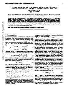
(x, y) ∈ Ω = [0, 1000] × [0, 1000], with the first order boundary conditions (2). We assume that α = 0. The coefficient k(x, y) is given by k(x, y) = 2π fl/c (x, y) where c (x, y) is presented in the Fig. 4. The grid size satisfies the condition 1 maxx (k(x))h = 0.625, where h = N − . The solution for the model problem (13) for f = 30 Hz is given in Fig. 5. 1

H. Knibbe et al. / Journal of Computational and Applied Mathematics 236 (2011) 281–293

Fig. 3. The solution of the model problem MP1 (12) for k = 40.

0 100 2000 m/s

200 Depth (m)

300 400 500

1500 m/s

600 700 800

3000 m/s

900 1000

0

200

400

600

800

1000

x (m) Fig. 4. The velocity profile of the wedge problem MP2.

Fig. 5. Real part of solution of the wedge problem MP2, f = 30 Hz.

289

290

H. Knibbe et al. / Journal of Computational and Applied Mathematics 236 (2011) 281–293 Table 6 Timing for 100 iterations of Bi-CGSTAB and IDR(s), s = 4, for k = 40 and different grid sizes. N

64 128 256 512 1024

Bi-CGSTAB

IDR(s)

tCPU (s)

tGPU (s)

Speedup

tCPU (s)

tGPU (s)

Speedup

0.5 2.3 8.9 33.0 130.4

0.07 0.1 0.2 0.9 3.2

7.8 21.1 35.8 35.3 40.6

1.3 5.3 23.4 124.5 363.2

0.36 0.47 0.89 2.6 9.5

3.7 11.3 26.1 47.8 38.3

4.1. Hardware and software specifications Before we start to describe the convergence and timing results, it is necessary to detail the hardware specifications. The experiments have been run on an AMD Phenom(tm) 9850 Quad-Core Processor, 2.5 GHz with 8 GB memory. Further we refer either to a single CPU or to a Quad-Core (4 CPUs). The compiler on CPU is gcc 4.3.3. The graphics card is an NVIDIA GeForce 9800 GTX/9800 GTX+, compute capability 1.1, 128 cores, 512 MB global memory, clock rate 1.67 GHz. The code on GPU has been compiled with NVIDIA CUDA 3.1.1 4.2. Bi-CGSTAB and IDR(s) We first consider the timings characteristics of Bi-CGSTAB and IDR(s) methods described in Section 2.3 and compare their performance on a single-threaded CPU against a GPU implementation. In both cases single precision has been used; see Table 6. We have chosen the number of iterations equal to 100, because even for relatively small wave numbers like k = 40 Bi-CGSTAB and IDR(s) do not converge. To achieve convergence a preconditioner should be used; see Section 4.3. For IDR(s) we use s = 4 normally distributed random vectors, that are orthogonalized by the Gram–Schmidt orthogonalization technique. As it is shown in Table 6, the speedups for Bi-CGSTAB and IDR(s) on GPU are comparable. It means that the IDR(s) is parallelizable and suitable for the GPU in a similar way as Bi-CGSTAB. Note that the timings for IDR(s) on CPU (s = 4) are approximately three times slower than the timing for Bi-CGSTAB on CPU. The reason for this is that the IDR(4) algorithm has 5 SpMVs (Sparse Matrix-Vector-Products) and dot-products per iteration and Bi-CGSTAB has only 2 of them per iteration, which gives a factor 2.5. Moreover, in the current implementation the preconditioned IDR(s) algorithm is applied (see Algorithm 1 or [6]), where as the ‘‘preconditioner‘‘the identity matrix is used. With additional optimizations of the current implementation, the factor 2.5 between Bi-CGSTAB and IDR(s) (s = 4) on CPU can be achieved. 4.3. Preconditioned Krylov methods 4.3.1. Bi-CGSTAB preconditioned by shifted Laplace multigrid Since neither Bi-CGSTAB nor IDR(s) converge as stand-alone solvers even for small wave numbers, a preconditioner is required to improve the convergence properties. As a preconditioner we apply the shifted Laplace multigrid method described in Section 4.3. Parameter β1 is set to 1. The idea is to choose such a combination of the parameter β2 and the relaxation parameter ω for the smoother that the number of iterations of Krylov methods will be reduced. Several smoothers are considered: damped Jacobi (ω-Jacobi), multi-colored Gauss–Seidel and damped multi-colored Gauss–Seidel (ω-Gauss–Seidel). Two-dimensional convergence results, in dependence of parameter β2 , for problem size N = 1024 are given in the Fig. 6. The results have been computed using Bi-CGSTAB in double precision on CPU with the preconditioner on a GPU. It can be clearly seen that using damped multi-colored Gauss–Seidel (ω = 0.9) as a smoother and β2 = 0.6 in the shifted Laplace multigrid preconditioner gives the minimum number of iterations of Bi-CGSTAB. In our further experiments those parameters are applied. By solving the MP1 (12) with Bi-CGSTAB preconditioned by one F -cycle of the shifted Laplace multigrid method, the following results have been achieved; see Table 7. The parameters are β1 = 1, β2 = 0.6. As a smoother the damped multicolored Gauss–Seidel with ω = 0.9 has been applied (4 colors). The grid sizes for different k satisfy the condition kh = 0.625. The implementation on the CPU is in double precision whereas on the GPU it is in single precision. Note that the number of iterations on CPU and GPU is comparable. A stopping criterion of ‖r ‖/‖r0 ‖ = 10−3 allows Bi-CGSTAB to converge on CPU and GPU so that performance comparisons can be made. In Table 7 we compare the preconditioned solver on CPU and GPU as well as the solver on CPU preconditioned by the multigrid method implemented on GPU. The idea behind this last implementation is to use the GPU as an accelerator for the preconditioner while we can maintain accuracy by the double precision solver on the CPU. However in this case the data

1 On different hardware we observed no significant differences in execution times between CUDA 3.1 and CUDA 3.2 for our software.

H. Knibbe et al. / Journal of Computational and Applied Mathematics 236 (2011) 281–293

800

0.4–Jacobi GS 0.5–GS 0.6–GS 0.7–GS 0.8–GS 0.9–GS

750 700 650 #iterations

291

600 550 500 450 400 350 300 0.4

0.5

0.6

0.7 beta2

0.8

0.9

1

Fig. 6. Comparison of number of iterations of Bi-CGSTAB preconditioned by shifted Laplace multigrid preconditioner with various β2 and different smoothers: damped Jacobi (ω = 0.4), Gauss–Seidel and damped Gauss–Seidel (ω = 0.5, 0.6, 0.7, 0.8, 0.9). Table 7 Timing comparisons of Bi-CGSTAB preconditioned by one F -cycle of the shifted Laplace multigrid method on single CPU and single GPU for MP1 (12), kh = 0.625. The combination of methods on single CPU (double precision) and single GPU (single precision) is also presented. N

k

64 128 256 512 1024

40 80 160 320 640

BiCGSTAB(CPU) + MG(CPU)

Bi-CGSTAB(CPU) + MG(GPU)

Bi-CGSTAB(GPU) + MG(GPU)

#iter

Time (s)

#iter

Time (s)

Speedup

#iter

Time (s)

Speedup

12 21 40 77 151

0.3 1.9 15.1 115.1 895.1

12 21 40 78 160

0.2 0.9 4.4 28.6 218.8

1.5 2.1 3.4 4.0 4.1

12 21 40 72 157

0.2 0.5 1.5 5.3 31.1

1.3 3.8 10.03 21.7 28.8

Table 8 Convergence of Bi-CGSTAB preconditioned by one F -cycle of the shifted Laplace multigrid method on single CPU and single GPU for MP2 (13), max(k)h = 0.625. Note that here Bi-CGSTAB on the CPU is in double precision. N

1024

Bi-CGSTAB(CPU) + MG(CPU)

Bi-CGSTAB(CPU) + MG(GPU)

#iter

Time (s)

#iter

Time (s)

Speedup

Bi-CGSTAB(GPU) + MG(GPU) #iter

Time (s)

Speedup

27

155

38

57

2.7

26

5.6

27.7

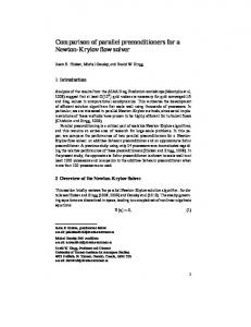
transfer (residual and solution) between CPU and GPU reduces the benefits of GPU implementation. If all data stays on the GPU as for Bi-CGSTAB preconditioned by multigrid on GPU, we find a much better speedup. We also solved the wedge problem MP2 (13) with Bi-CGSTAB on the CPU preconditioned by the shifted Laplace multigrid method on the GPU. The parameters in the preconditioner are β1 = 1 and β2 = 0.6. The relaxation parameter for the multicolored Gauss–Seidel is ω = 0.9. The results are shown in Table 8. As stopping criterion ‖r ‖/‖r0 ‖ = 10−3 is used. 4.3.2. IDR(s) preconditioned by shifted Laplace multigrid By solving MP1 (12) with IDR(s) preconditioned by one F -cycle of the shifted Laplace multigrid method, the following results have been achieved; see Table 9. We use s = 4 normally distributed random vectors, which are orthogonalized by the Gram–Schmidt orthogonalization technique. As a smoother a multi-colored Gauss–Seidel has been applied. In order to obtain an optimal number of iterations for IDR(s), we have used the same procedure to find optimal β2 = 0.65 and ω = 0.9 as described in Section 4.3.1. The grid sizes for different k satisfy the condition kh = 0.625. The implementation on the CPU is in double precision and on the GPU is in single precision. As stopping criterion again ‖r ‖/‖r0 ‖ = 10−3 is used. The convergence curves of IDR(s) compared with Bi-CGSTAB are shown in Fig. 7, where the horizontal axis represents the number of iterations. In this case we use Krylov methods in double precision on a CPU with the preconditioner on a GPU. One iteration of Bi-CGSTAB contains 2 SpMVs (short for Sparse Matrix-Vector-Multiplication), whereas one iteration of IDR(4) contains 5 SpMVs. From Fig. 7 it is easy to see that the total number of SpMVs for Bi-CGSTAB and IDR(4) is the same. The fact that the IDR(s) method converges in fewer iterations, but has more SpMVs, implies that the total performance of IDR(4) and Bi-CGSTAB is approximately the same.

292

H. Knibbe et al. / Journal of Computational and Applied Mathematics 236 (2011) 281–293

Table 9 Timing comparisons of IDR(s) preconditioned by one F -cycle of the shifted Laplace multigrid method on single CPU and single GPU for MP1 (12), kh = 0.625. The combination of methods on single CPU (double precision) and single GPU (single precision) is also presented. N

64 128 256 512 1024

k

40 80 160 320 640

IDR(s)(CPU) + MG(CPU)

IDR(s)(CPU) + MG(GPU)

#iter

Time (s)

#iter

Time (s)

Speedup

IDR(s)(GPU) + MG(GPU) #iter

Time (s)

Speedup

6 10 17 33 69

0.36 2.3 15.8 126.7 1061.8

6 10 17 34 68

0.32 1.04 4.65 33.1 252.2

1.1 2.2 3.3 3.8 4.2

6 10 18 33 73

0.27 0.7 1.7 6.1 37.3

1.3 3.7 9.1 20.6 28.5

10 1

Bi–CGSTAB CPU prec CPU Bi–CGSTAB CPU prec GPU Bi–CGSTAB GPU prec GPU IDR(4) CPU prec CPU IDR(4) CPU prec GPU IDR(4) GPU prec GPU

10 0 L2–norm residual

10 –1 10 –2 10 –3 10 –4 10 –5 10 –6 10 –7

0

50

100 150 #iterations

200

250

Fig. 7. Convergence curves of IDR(4) and Bi-CGSTAB for the model problem MP1 (12) for k = 320. Table 10 Convergence of IDR(s) preconditioned by one F -cycle of the shifted Laplace multigrid method on single CPU and single GPU for MP2 (13), max(k)h = 0.625. Note that here the IDR on the CPU is in double precision. N

1024

IDR(s)(CPU) + MG(CPU)

IDR(s)(CPU) + MG(GPU)

#iter

Time (s)

#iter

Time (s)

Speedup

IDR(s)(GPU) + MG(GPU) #iter

Time (s)

Speedup

11

162.9

12

43.9

3.7

12

6.3

25.7

We solve the wedge problem MP2 (13) with the IDR(s) on the CPU preconditioned by the shifted Laplace multigrid method on the GPU. The parameters in the preconditioner are β1 = 1 and β2 = 0.65. The relaxation parameter for the multicolored Gauss–Seidel is ω = 0.9. The same stopping criterion ‖r ‖/‖r0 ‖ = 10−3 is used. The results are shown in Table 10. 5. Conclusions In this paper we have presented a GPU implementation of Krylov solvers preconditioned by a shifted Laplace multigrid preconditioner for a two-dimensional Helmholtz equation. On CPU, double precision was used whereas on a GPU computations were in single precision. We have seen that Bi-CGSTAB and IDR(s) are parallelizable on GPU and have similar speedups of about 40 compared to a single-threaded CPU implementation. It has been shown that a matrix-dependent multigrid can be implemented efficiently on GPU where a speedup of 20 can be achieved for large problems. As the smoother we have considered parallelizable methods such as weighted Jacobi (ω-Jacobi), multi-colored Gauss–Seidel and damped multi-colored Gauss–Seidel (ω-GS). Parameter β2 = 0.6 in the preconditioner is optimal for damped multi-colored Gauss–Seidel smoother with ω = 0.9. With those parameters, the number of iterations is optimal for Bi-CGSTAB. For IDR(s) the optimal parameters were β2 = 0.65 and ω = 0.9. One iteration of preconditioned IDR(s) is more intensive than one iteration of preconditioned Bi-CGSTAB, however IDR(s) needs fewer iterations so it does not affect the total computation time. To increase the precision of a solver, iterative refinement has been considered. We have shown that iterative refinement with Bi-CGSTAB on GPU is about 4 times faster than Bi-CGSTAB on CPU for the same stopping criterion. The same result has been achieved for IDR(s). Moreover, combinations of Krylov solvers on CPU and GPU and the shifted Laplace multigrid preconditioner on CPU and GPU are considered. A GPU Krylov solver with a GPU preconditioner give the best speedup. For

H. Knibbe et al. / Journal of Computational and Applied Mathematics 236 (2011) 281–293

293

example for the problem size n = 1024 × 1024 Bi-CGSTAB on GPU with the GPU preconditioner as well as IDR(s) on GPU with the GPU preconditioner are about 30 times faster than the analogous solvers on CPU. The GPU implementation of a Helmholtz Krylov solver preconditioned by a shifted Laplace preconditioner can be generalized to three dimensions, which is one of the aspects of the current work. Other aspects will include multi-core CPUs and multi-GPUs as well. Acknowledgments The authors would like to thank the referees for the reading of the manuscript and the helpful comments. References [1] Nvidia CUDATM , programming guide, version 2.2.1, 2009. http://developer.download.nvidia.com/compute/cuda/2_21/toolkit/docs/NVIDIA_CUDA_ Programming_Guide_2.2.1.pdf. [2] K. Karimi, N.G. Dickson, F. Hamze, A performance comparison of CUDA and Open CL, Int. J. High Perform. Comput. Appl., 2011. doi:10.1177/1094342010372928. [3] P. Du, P. Luszczek, J. Dongarra, OpenCL evaluation for numerical linear algebra library development, in: Symposium on Application Accelerators in High-Performance Computing, SAAHPC’10, 2010. [4] Y.A. Erlangga, A robust and efficient iterative method for the numerical solution of the Helmholtz equation, Ph.D. Thesis, Delft University of Technology, The Netherlands, 2005. [5] H.A.V. der Vorst, Bi-CGSTAB: a fast and smoothly converging variant of Bi-CG for the solution of nonsymmetric linear systems, SIAM J. Sci. Stat. Comput. 13 (1992) 631–644. [6] P. Sonneveld, M.B. van Gijzen, IDR(s): a family of simple and fast algorithms for solving large nonsymmetric systems of linear equations, SIAM J. Sci. Comput. 31 (2) (2008) 1035–1062. [7] J. Gozani, A. Nachshon, E. Turkel, Conjugate gradient coupled with multigrid for an indefinite problem, in: Advances in Comput. Methods for PDEs, vol. V, 1984, pp. 425–427. [8] R. Kechroud, A. Soulaimani, Y. Saad, S. Gowda, Preconditioning techniques for the solution of the Helmholtz equation by the finite element method, Math. Comput. Simulation 65 (4–5) (2004) 303–321. doi:10.1016/j.matcom.2004.01.004. [9] A.L. Laird, M.B. Giles, Preconditioned iterative solution of the 2D Helmholtz equation, Tech. Rep. 02/12, Oxford Computer Laboratory, Oxford, UK, 2002. [10] E. Turkel, Numerical methods and nature, J. Sci. Comput. 28 (2006) 549–570. [11] Y.A. Erlangga, C. Vuik, C.W. Oosterlee, On a class of preconditioners for solving the discrete Helmholtz equation, in: G. Cohen, E. Heikkola, P. Joly, P. Neittaanmakki (Eds.), Mathematical and Numerical Aspects of Wave Propagation, Univ. Jyväskylä, Finnland, 2003, pp. 788–793. [12] Y.A. Erlangga, C.W. Oosterlee, C. Vuik, A novel multigrid based preconditioner for heterogeneous Helmholtz problems, SIAM J. Sci. Comput. 27 (2006) 1471–1492. [13] Y.A. Erlangga, C. Vuik, C. Oosterlee, On a class of preconditioners for solving the Helmholtz equation, Appl. Numer. Math. 50 (2004) 409–425. [14] V.W. Lee, C. Kim, J. Chhugani, M. Deisher, D. Kim, A.D. Nguyen, N. Satish, M. Smelyanskiy, S. Chennupaty, P. Hammarlund, R. Singhal, P. Dubey, Debunking the 100× GPU vs. CPU myth: an evaluation of throughput computing on CPU and GPU, SIGARCH Comput. Archit. News 38 (3) (2010) 451–460. doi:10.1145/1816038.1816021. [15] 2010. www.nvidia.com. [16] M. Baboulin, A. Buttari, J. Dongarra, J. Kurzak, J. Langou, J. Langou, P. Luszczek, S. Tomov, Accelerating scientifing computations with mixed precision algorithms, http://dblp.uni-trier.de/db/journals/corr/corr0808.html, CoRR, abs/0808.2794. [17] R. Clayton, B. Engquist, Absorbing boundary conditions for acoustic and elastic wave equations, Bull. Seismol. Soc. Amer. 67 (6) (1977) 1529–1540. [18] B. Engquist, A. Majda, Absorbing boundary conditions for numerical simulation of waves, Math. Comp. 31 (1977) 629–651. [19] Y. Saad, Iterative Methods for Sparse Linear Systems, SIAM, Philadelphia, 2003. [20] M.B. van Gijzen, Y.A. Erlangga, C. Vuik, Spectral analysis of the discrete Helmholtz operator preconditioned with a shifted Laplace, SIAM J. Sci. Comput. 29 (2007) 1942–1958. [21] P. Wesseling, P. Sonneveld, Numerical experiments with a multi-grid and a preconditioned Lanczos type method, Lecture Notes in Math. 771 (1980) 543–562. [22] M.B. van Gijzen, P. Sonnenveld, An elegant IDR(s) variant that efficiently exploits bi-orthogonality properties, ACM Trans. Math. Softw, 2010. [23] N. Umetani, S.P. MacLachlan, C.W. Oosterlee, A multigrid-based shifted Laplacian preconditioner for a fourth-order Helmholtz discretization, Numer. Linear Algebra Appl. 16 (2009) 603–626. [24] H.R. Elman, O.G. Ernst, D.P. O’Leary, A multigrid method enhanced by Krylov subspace iteration for discrete Helmholtz equations, SIAM J. Sci. Comput. 23 (2001) 1291–1315. [25] P.M. de Zeeuw, Matrix-dependent prolongations and restrictions in a blackbox multigrid solver, J. Comput. Appl. Math. 33 (1990) 1–27. [26] A. Fog, Instruction tables: List if instruction latencies, throughputs and micro-operation breakdowns for Intel, AMD and VIA CPUs, Copenhagen University College of Engineering. [27] G. Golub, C. van Loan, Matrix Computations, 3rd ed., The Johns Hopkins University Press, Baltimore, 1996. [28] J.M. Elble, N.V. Sahinidis, P. Vouzis, GPU computing with Kaczmarz’s and other iterative algorithms for linear systems, Parallel Comput. 36 (2010) 215–231. [29] R.E. Plessix, W.A. Mulder, Separation-of-variables as a preconditioner for an iterative Helmholtz solver, Appl. Numer. Math. 44 (3) (2003) 385–400.