gpuSPHASE—A shared memory caching ... - CyberLeninka

Computer Physics Communications (

)

–

Contents lists available at ScienceDirect

Computer Physics Communications journal homepage: www.elsevier.com/locate/cpc

gpuSPHASE—A shared memory caching implementation for 2D SPH using CUDA✩ Daniel Winkler ∗ , Michael Meister, Massoud Rezavand, Wolfgang Rauch Unit of Environmental Engineering, University of Innsbruck, Technikerstrasse 13, 6020, Innsbruck, Austria

article

info

Article history: Received 12 November 2015 Received in revised form 8 November 2016 Accepted 29 November 2016 Available online xxxx Keywords: Computational fluid dynamics CUDA GPGPU GPU Smoothed particle hydrodynamics

abstract Smoothed particle hydrodynamics (SPH) is a meshless Lagrangian method that has been successfully applied to computational fluid dynamics (CFD), solid mechanics and many other multi-physics problems. Using the method to solve transport phenomena in process engineering requires the simulation of several days to weeks of physical time. Based on the high computational demand of CFD such simulations in 3D need a computation time of years so that a reduction to a 2D domain is inevitable. In this paper gpuSPHASE, a new open-source 2D SPH solver implementation for graphics devices, is developed. It is optimized for simulations that must be executed with thousands of frames per second to be computed in reasonable time. A novel caching algorithm for Compute Unified Device Architecture (CUDA) shared memory is proposed and implemented. The software is validated and the performance is evaluated for the well established dambreak test case. Program summary Program title: gpuSPHASE Catalogue identifier: AFBO_v1_0 Program summary URL: http://cpc.cs.qub.ac.uk/summaries/AFBO_v1_0.html Program obtainable from: CPC Program Library, Queen’s University, Belfast, N. Ireland Licensing provisions: GNU GPLv3 No. of lines in distributed program, including test data, etc.: 128288 No. of bytes in distributed program, including test data, etc.: 1350326 Distribution format: tar.gz Programming language: C++, CUDA. Computer: Nvidia CUDA capable devices. Operating system: Linux, Windows, Mac OS. Classification: 5, 12. External routines: Qt5 Core, HDF5, H5Part Nature of problem: Free surface fluid dynamics simulations of long running physical phenomena that must be calculated in the order of real-time.

✩ This paper and its associated computer program are available via the Computer Physics Communication homepage on ScienceDirect (http://www.sciencedirect.com/ science/journal/00104655). ∗ Corresponding author. E-mail address: [email protected] (D. Winkler).

http://dx.doi.org/10.1016/j.cpc.2016.11.011 0010-4655/© 2016 The Author(s). Published by Elsevier B.V. This is an open access article under the CC BY license (http://creativecommons.org/licenses/by/4.0/).

2

D. Winkler et al. / Computer Physics Communications (

)

–

Solution method: gpuSPHASE is a 2D SPH solver for CUDA capable devices that is optimized for the computation of real-time simulations. Running time: Depending on the simulated problem the running time varies from seconds to weeks. © 2016 The Author(s). Published by Elsevier B.V. This is an open access article under the CC BY license (http://creativecommons.org/licenses/by/4.0/).

1. Introduction Smoothed particle hydrodynamics (SPH) is a meshless particle based method that has initially been independently introduced by Lucy [1] and Gingold and Monaghan [2] for solving astrophysical problems. The general concept is the discretization of a continuous medium into interpolation points known as particles to transform partial differential equations into an integral form. Using integral interpolation theory the particles’ properties are evolved in time based on the properties of neighboring particles [3]. Following this concept, the main advantages over mesh based approaches arise from the inherent Lagrangian nature, because the method follows the particles as they move through space and time. This allows to accurately simulate free surface evolution without topological restrictions, multi-phase interfaces in highly dynamic flows, fluid–structure interactions and multi-phase phenomena. Given the numerous advantages over grid based methods, SPH has been applied to a manifold of application domains, such as magnetohydrodynamics [4], solid mechanics [5–8], computational fluid dynamic [9,3] and many other multi-physics problems [10–12]. A well known property of simulating transient flows in engineering problems is the high computational demand that arises in solving the Navier Stokes equations, which applies to Eulerian as well as to Lagrangian methods. The computational effort can be reduced in SPH by limiting the amount of neighbors used for interpolation, but the cost still requires high performance computing (HPC) for practical applications. In recent years general purpose computation on graphics processing units (GPGPU) emerged as a technique to use the high floating point arithmetic performance of graphics devices for general purpose calculations. This paradigm creates the possibility to execute simulations on GPU computing workstations that required HPC clusters before. For this reason a lot of SPH solvers have been developed that harness the computational power of GPUs. Two established open-source GPU implementations are GPUSPH [13] and DualSPHysics [14]. Both implementations originated from the serial CPU based SPHysics code [15] that has initially been released in 2007. The main difference between the two implementations is that GPUSPH supports 3-D simulations only and uses a neighbor list for each particle for several iterations. It is shown in [16] that this approach results in a significantly lower number of maximum particles and causes no performance improvement over DualSPHysics for several test cases. Since both implementations require Nvidia GPUs to be executed AQUAgpusph [16] has been implemented using the open standard OpenCL so that accelerator cards from vendors such as Nvidia, AMD, Intel and IBM can be used. While the maximum performance is also worse than DualSPHysics, the versatility in hardware allows for the best performance to cost ratio. It has to be noted that DualSPHysics additionally provides an optimized CPU version that does not require an accelerator card and can thus be executed on any desktop or workstation computer. The implementation uses OpenMP to achieve a high performance for many core shared memory architectures.

A major challenge when simulating transport phenomena prevalent in biological and chemical engineering is the difference in the temporal scales. To generate meaningful results of the effects of hydraulics on environmental processes several weeks of physical time need to be simulated [17,18]. Contrary, simulating fluids with weakly compressible SPH with a coarse resolution requires time steps in the order of 10−4 s, such that 108 –1010 iterations are needed. Every such iteration involves calculating the force exerted on each particle within the simulation domain. Performing these simulations in 3D requires decades of computation time on high end graphics devices [14]. Employing the multi-GPU capabilities of solvers like DualSPHysics [19] and GPUSPH [20] reduces the computational time, but the time necessary for synchronization of problems that require billions of iterations still prevents computation in feasible time. The compromise to cope with such simulations is to reduce the complexity of the simulation by constraining it to two dimensions and reduce the spatial resolution [17]. From this restriction arise possibilities for algorithmic optimizations in the implementation. This paper describes gpuSPHASE, a GPU accelerated general purpose SPH solver created for solving two dimensional hydrodynamic problems. The implementation reduces the computational effort by implementing well established techniques like space filling curves and a neighborhood list. Generic methods to optimize the execution pipeline and data layout are described and evaluated to improve the performance of gpuSPHASE. A novel caching algorithm to accelerate the calculation of unstructured neighborhood problems using the CUDA shared memory cache is presented and analyzed. Validation of the implementation is performed and evaluated for different established test cases. The simulation performance for the well established dambreak test case is compared to the high performance SPH solver DualSPHysics. It is shown that the caching algorithm produces a very good speedup compared to a hardware caching approach and that the overall performance of the solver is very good. 2. Numerical method SPH was introduced individually by Lucy [1] and Gingold and Monaghan [2] as a method for solving astrophysical problems. Since then the method has been applied to other fields like solid mechanics, magnetodynamics and fluid mechanics where reliable results were achieved. Key advantages of the method are the straight forward handling of multi-phase flows and the natural computation of the free surface [3]. 2.1. Kernel function As the name smoothed particle hydrodynamics indicates the method is based on particles. These particles are interpolation points that represent the continuum and as such move with the simulated fluid. The force calculation that imposes the advection of the particles is based on the properties of neighboring particles. By using a kernel function W the influence of the neighbor properties is weighted depending on the distance r. The kernel has to fulfill

D. Winkler et al. / Computer Physics Communications ( n+ 21

the property



W (r, h) dr = 1

)

∆t

ri

= rni +

ρ

= ρ + ∆t

2

(1)

but due to computational properties it is preferable to add another constraint on the support of the kernel rc = κ h so that W (|r| > rc , h) = 0.

(2)

The combination of a suitable kernel function with a limited support ensures that the number of neighbors incorporated in the calculation is low enough to make correct but computationally feasible calculations [21]. 2.2. Continuity equation

–

3

n+ 12

vi

(8)

n+ 12

n +1 i

n i

n+ 21

rni +1 = ri

n+ 12

vin+1 = vi

dρi

(9)

dt

+

∆t

+

∆t

2

n+ 12

vi



(10)

dvi

2

 n +1 (11)

dt

which is a second order accurate symplectic mid-step scheme. The continuity equation (9) and the force computation (11) are the computationally most expensive parts and need only be performed once per step. The time step is limited by several conditions, where the CFL condition [3] is usually the most restrictive

The first governing equation for fluid dynamics is the continuity equation, which relates the change of density to the advection of the continuum.

∆t 6

dρ

Additionally the viscous condition

= −ρ∇ · v.

dt

(3)

The variables t, ρ and v represent the time, density and velocity, respectively. When applied to SPH the equation can be discretized for a reference particle i using the kernel function W dρ i

= ρi

dt

 mj

vij · ∇i Wij

ρj

j

(4)

∆t 6

h

1

4 cmax + |vmax |

.

(12)

1 h2

(13)

8 ν

and the body force condition

∆t 6

1



h

1/2 (14)

|g|

4

where mj denotes the mass, vij = vi − vj expresses the relative velocity and ∇i Wij = ∇i W (ri − rj , h) the gradient of the kernel weight function for the neighbor particles j [3].

need to be fulfilled.

2.3. Momentum equation

Solid boundary conditions based on boundary particles can handle arbitrary shapes and geometries in two and three dimensions. The particles are statically positioned and evolve the pressure based on the surrounding fluid particles. This pressure is included in the force computation of the fluid particles to enforce the impermeability condition of the wall. The discretized calculation of the pressure of a wall particle w is defined by the neighboring fluid particles f [22]

The second governing equation is the momentum equation

ρ

dv

= −∇ p + F(ν) + ρ g

dt

(5)

with p denoting the pressure, F(ν) the viscous and g the body force. gpuSPHASE uses the weakly compressible formulation of SPH (WCSPH) and we refer to [3] for further details on the equations. The momentum equation, including artificial viscosity and the acceleration caused by shear forces, is discretized to [22] dvi dt

=−

 ρj pi + ρi pj 1  2 Vi + Vj2 ∇i Wij mi j ρi + ρj

(momentum)

vij · rij ∇i Wij (viscosity)  2 ρij (rij  + ϵ h2ij ) j  vij ∂ W 1  2ηi ηj  2 + Vi + Vj2 (shear forces) (6) mi j ηi + ηj rij ∂ rij   where rij = ri − rj , rij = rij  and ∂ W /∂ rij = ∇i Wij · eij . The coefficients hij , cij and ρij are the smoothing length, speed of



−

mj α hij cij

sound and density averaged between two particles. Variables Vi and ηi represent the volume and dynamic viscosity of particle i, the quantifier ϵ = 0.01 is included to ensure a non-zero denominator. 2.4. Time stepping The time integration uses the velocity-Verlet scheme [23] n+ 21

vi

=

vni

+

∆t 2



dvi dt

n (7)

2.5. Solid boundary conditions

 pw =

f

pf Wwf + (g − aw ) ·



f

Ww f



f

ρ f rw f W w f

.

(15)

A computational advantage of this method is the straight-forward implementation of the method as it solely adds another calculation step following the particle principle. From the implementation point of view the existing data structures are reused and Eq. (15) is applied such that the parallel nature of the algorithm is retained. 3. Implementation The main goal in the gpuSPHASE implementation is to have a fast and versatile two dimensional SPH solver that can be reused for different fields of application in engineering. The solver is designed as a standalone component that can be executed on any CUDA capable platform. It is optimized for long running simulations but can be applied to solve any problem with 2D WCSPH. Although there are already a number of language bindings available for CUDA we use C++ as it is the most common one. C++ has been used in HPC for decades as it provides a good compromise between abstraction and flexibility. The open-source Qt5 framework facilitates platform independent abstractions for data input and output. The program uses a custom input format encoded in the JSON format, which is easy to read and edit in a

4

D. Winkler et al. / Computer Physics Communications (

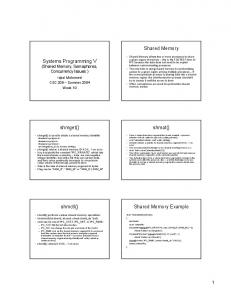
standard text editor. To store particle configurations to disk the H5Part format and library are used. These interfaces allow users to easily configure the scene that has to be simulated and use the results in other software applications. 3.1. CUDA function execution pipeline Since the implementation of this new solver aims at performance improvements this section elaborates on the implementation of the CUDA kernels. Due to the name conflict of the SPH kernel with CUDA kernel we will use the term CUDA function to refer to a CUDA kernel from here on. Fig. 1 shows the dependency graph for the CUDA functions used in gpuSPHASE. It visualizes data nodes with ellipses, CUDA functions with rectangles and dependencies with arrows. The light green coloring depicts CUDA functions with less strict execution dependencies, which means that those functions may be executed in parallel to the main pipeline. Some data nodes are duplicated to avoid arrows cluttering the graph but equal names refer to the same memory locations. The suffixes _L and _R denote two different memory arrays for the same data. E.g. the CUDA function accelerate needs the velocity and force data v_L and f_L as input and writes the new velocity data to v_R as output. Some of the functions strictly depend on the finished execution of the previous function, thus it is not possible to merge them into a single function. This restriction needs to be satisfied because of the data dependency to neighbor data, i.e. in order to calculate the continuity equation for a particle i, the position of all neighboring particles j have to be updated (cf. Section 2.4). That requirement can only be fulfilled by a global synchronization, which boils down to the separation of the computation into several CUDA functions. A major drawback of this splitting is that all data that has already been transferred to the GPU is discarded and has to be transferred again for the next CUDA function using the same data. Caching could help in this case but since the amount of data necessary for most simulations is much bigger than the cache size it is unlikely that there is a significant influence. Discarding all data demands to calculate the particle distances and kernel weights multiple times per iteration, but due to memory and bandwidth restrictions it is favored over storing the data explicitly. Because of the data dependency functions must store the new data values to a different location. gpuSPHASE solves this problem with double buffers that are swapped as soon as all new data is written. The use of two separate buffers decouples functions that are not data dependent such that they can be executed in parallel. E.g. particle positions may already be advanced to rin+1 in n+ 1

parallel to the continuity equation that uses ri 2 . Exception to this restriction is the extrapolation function since it writes boundary particle data and reads fluid particle data. This is marked with the asterisks symbol (∗) in the data nodes, which indicates that it is still the same array but some data has been updated. Reusing the same data location avoids bare copying of fluid particle data, which is beneficial for the performance of the function. Although some degree of execution parallelism is possible, performance is worse when leveraging it with the usage of CUDA streams for rather small simulations. This is caused by the synchronization overhead combined with the high number of function executions per second. A promising optimization approach is the combination of several distinct data arrays into a single one [24]. CUDA provides vector types that combine up to four single precision floating point values into a single one. Since x and y positions are mainly used in combination, it is obvious to combine the two elements into a single value of type float2. This allows the CUDA run-time to load both values at once instead of retrieving it from two different

)

–

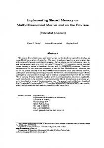
memory locations. Less obvious but similar is the combination of particle properties into a vector type as those properties depend on one another and often all of them are required as input and output to a CUDA function. Fig. 2 shows an optimized workflow where data arrays have been vectorized such that less data nodes are necessary. Apart from the force f and the auxiliary c_max and v_max arrays, the data has been combined into float4 data arrays

• motion consisting of position r and velocity v • traits consisting of pressure p, density rho, volume vol and speed of sound c. Analyzing the dependencies enforced by the time stepping scheme described in Section 2.4, steps (7), (8) and (10) are n+ 1

n+ 1

combined into a single function. Using ri 2 and vi 2 it is possible to calculate the continuity equation, the force calculation in step (11) requires the positions rin+1 . Thus the input data array is used n+ 1

to store rin+1 and vi 2 , which is the data required for calculating the extrapolation and momentum functions. Furthermore the acceleration (11) is calculated in the momentum function, which removes another CUDA function call. Apart from the reduced overhead of launching CUDA functions and removing global synchronization, increasing the tasks that are performed in every function reduces the amount of data that has to be transferred. While the momentum equation in the nonoptimized workflow stores the calculated force to memory and the accelerate function has to load it, merging the two functions no longer requires the data to be loaded from global memory. The implementation of vector types makes this optimization even more important. 3.2. Shared memory caching algorithm While modern GPUs provide peak computing performance of several trillion floating point operations per second (TFLOPS) the efficiency of real world applications is often much lower. For many applications the memory bandwidth and latency are a bottleneck, which can be improved with intelligent design and performance profiling. For details we refer to the CUDA C Programming Guide [24]. The main problem for memory bound applications is that the CUDA global memory is not fast enough to provide data to the compute units. CUDA tries to compensate this deficiency by executing several threads per processor in parallel. Based on hardware limitations and the complexity of the CUDA function the amount of threads per processor is limited, which is referred to as occupancy [24]. Another important aspect of memory is the order in which it is accessed. Ideally all data is loaded in a coalesced fashion, which means that every consecutive thread loads data from a consecutive memory address. While this seems easy for methods that access ordered data, there is no obvious way to do so in an unordered scheme like SPH. No efficient data structure exists to arrange the neighbor data in memory so that it can be read coalesced unless all neighbor data is redundantly stored for every particle. gpuSPHASE handles this issue with a novel algorithm that uses a two step loading mechanism. In a first step the relevant particle data is loaded to a very fast programmable cache in a coalesced fashion and after that the data is accessed in an irregular way, which has a much lower implication on the performance. Due to the unstructured nature of the SPH method, it is not possible to efficiently load all necessary data to the programmable cache. The following section outlines an approach that combines several techniques to optimize the data access.

D. Winkler et al. / Computer Physics Communications (

)

–

5

Fig. 1. CUDA function pipeline. Rectangles, circles and arrows denote CUDA functions, data arrays and dependencies, respectively. The bright green color indicates that the functions can be executed in parallel to the main pipeline. The asterisk marks data arrays that are read and written by a function. (For interpretation of the references to colour in this figure legend, the reader is referred to the web version of this article.)

3.2.1. Data layout using space filling curves Most existing implementations mention neighbor search as a key component of the SPH method implementation [19,16]. Referring to those works the most efficient implementation for this problem is to partition the particles into a unigrid [25]. This means that the entire domain is split up into equally sized cells and the particles are classified by the unique cell identifier they geometrically belong to. By choosing the cell dimension equal to – or greater than – the kernel support rc the grid gains the property that all neighbors j of a particle i are contained in the adjacent cells. This property holds for simulations in any geometric dimension d, resulting in 3d cells to check for neighbor particles.

In order to find the particles for a given cell in memory, the particle data needs to be sorted according to the cell identifier. After sorting a cell linked list is generated, which points to the beginning and end of every cell’s particles [25]. While the amount of particles to check is reduced drastically by this approach, those particles typically are spread across memory. This is an evident result as a higher dimensional problem is mapped to one dimensional memory. Space filling curves (SFC) are functions with the property to traverse higher dimensional space in a continuous fashion [26]. The Morton order [27] or Hilbert curve [28] are SFCs with good data locality characteristics, which means that for any two cells c1 and c2 that are geometrically close the function produces one dimensional indices H (xi , yi ) = ni that are ordinally

6

D. Winkler et al. / Computer Physics Communications (

)

–

Fig. 2. Optimized CUDA function pipeline. Rectangles, circles and arrows denote CUDA functions, data arrays and dependencies, respectively. The bright green color indicates that the functions can be executed in parallel to the main pipeline. The asterisk marks data arrays that are read and written by a function. (For interpretation of the references to colour in this figure legend, the reader is referred to the web version of this article.)

close. Ordering the particle data according to the mapped cell index compensates the computational overhead with better data locality. Data locality has positive effects on hardware caching, so ideally the overall performance of this approach is better than the straight forward mapping to memory. Fig. 3 shows a Hilbert space filling curve where every line is a connection of two points that have to be interpreted as grid cells containing particle data. Two particles have been chosen to visualize the concept of data locality, the center points mark the particle abstraction into a grid cell, the surrounding circles visualize the relevant neighborhood. Neglecting the curve coloring and type, one can see that the two dimensional neighborhood is clustered into few coherent memory regions, which is beneficial for batch loading and caching performed by hardware caches. 3.2.2. CUDA shared memory Interpreting the solid blue line in Fig. 3 as the amount of data that fits into software manageable cache visualizes the advantage of the approach. The light gray particle can be calculated with all necessary data already cached and as such completely neglecting memory latencies. While the black dashed circle does not exhibit this property the ratio of particles that can be calculated from cached data may still be high. This section describes the memory and caching implementation of gpuSPHASE that has the memory perks explained above. Computer memory design is always a trade-off between size and speed. While hard disks provide vast amount of storage the speed is rather slow, caches and registers are several orders of magnitude faster but for economic reasons limited in size. For this

reason, modern computer hardware design relies on a hierarchy of different storage units to compensate for this problem. A typical computer consists of a hard disk, random access memory (RAM) and several levels of on-chip caches. This hierarchy is abstracted by the hardware and operating system so that a standard application does not need to take care where the data is stored. HPC applications are typically designed and optimized to leverage the most performance of the described hierarchy. This means that the program needs to be profiled, a process where dedicated tools are used to evaluate how the data is cached by the hardware. Since the hardware caching cannot be controlled, the program must be reverse engineered to make the caching perform as expected. The CUDA execution model also employs this hierarchy on graphics devices but additionally provides the possibility to manually manage a very fast but small cache. By enabling developers to manage the data cache CUDA provides a mechanism to use domain knowledge for the optimization of the program execution. The downside is that programs that do not use shared memory lose a portion of fast hardware cache. Particle computations mostly depend on data of neighboring particles, which means that an efficient caching is important for maximum compute performance. The unstructured nature of SPH has no obvious implementation of SM caching, even in combination with the memory layout optimization discussed in 3.2.1. Motivated by the property that SFCs allow for data locality we propose an algorithm that makes extensive use of the SM concept. The idea is to organize the data in global memory sorted by a SFC. Size limitations of the shared memory require to partition the data into smaller sets, given the properties of SFCs these chunks are selected to be as big as possible.

D. Winkler et al. / Computer Physics Communications (

)

–

7

Fig. 3. Hilbert space filling curve. Every line is a connection of two points that have to be interpreted as grid cells, the solid blue line denotes the amount of data that fits into CUDA shared memory. Particles are visualized with bold points, the kernel support is indicated by the surrounding circle. (For interpretation of the references to colour in this figure legend, the reader is referred to the web version of this article.)

The CUDA architecture abstracts the execution of millions of threads. These threads are grouped into blocks that are distributed to the Streaming Multiprocessors (SMP) where they are executed isolated from other blocks. Within one block all threads can be synchronized and access CUDA shared memory. The size of the blocks must be selected depending on hardware restrictions and performance characteristics, a CUDA grid is used to organize and index the individual blocks. At this abstraction level the block size for gpuSPHASE functions is maximized with the requirement that at least two blocks must fit on an SMP. For the most recent CUDA architectures Kepler and Maxwell the resulting block sizes for the momentum function are 768 and 1024 threads, respectively. The limiting factors are the size of shared memory and the maximum number concurrent threads per SMP.

thread copies the particle data into the shared memory and waits for all other threads in the same block to do so. The code computing the interaction value is not different from a naïve implementation that reads all data from global memory (lines 11–15). The only prerequisite for this property is the pointer arithmetic on lines 6–10, which allows each thread to use manually cached data if available. This optimization is possible starting with the Nvidia Fermi architecture, where uniform addressing of shared and global memory space enables to decide at run-time which memory type is requested. Based on this feature gpuSPHASE limits branch divergence to the computation of memory addresses, but executes the physical calculations and data retrieval from different memory spaces in parallel. The result is that branch divergence is reduced to a minimum and the hardware hides the latency from global memory with occupancy.

Algorithm 1: Shared memory caching algorithm

1 2 3 4 5 6 7 8 9 10 11 12 13 14 15 16 17

Input: Thread index Input: Particle data pointer Input: Neighbor list Output: Interaction value Compute assigned particle index; Copy particle data to shared memory; Synchronize thread block; while neighbors in list do Choose neighbor from list; if neighbor in thread block then Initialize neighbor pointer to shared memory; else Initialize neighbor pointer to global memory; end Calculate distance; if distance