arXiv:1309.1226v1 [cs.AI] 5 Sep 2013
Graded Causation and Defaults∗ Joseph Y. Halpern† Cornell University
[email protected]
Christopher Hitchcock California Institute of Technology
[email protected]
September 6, 2013
Abstract Recent work in psychology and experimental philosophy has shown that judgments of actual causation are often influenced by consideration of defaults, typicality, and normality. A number of philosophers and computer scientists have also suggested that an appeal to such factors can help deal with problems facing existing accounts of actual causation. This paper develops a flexible formal framework for incorporating defaults, typicality, and normality into an account of actual causation. The resulting account takes actual causation to be both graded and comparative. We then show how our account would handle a number of standard cases.
1 Introduction The notion of actual causation (also called “singular causation”, “token causation”, or just “causation” in the literature), the relation that we judge to hold when we affirm a statement that one particular event caused another, is ubiquitous in descriptions of the world. For example, the following claims all describe relations of actual causation: • Paula’s putting poison in the tea caused Victoria to die. • A lightning strike caused the forest fire. ∗
For helpful comments and discussion, we would like to thank Luke Glynn, Franz Huber, Josh Knobe, Jonathan Livengood, Laurie Paul, Jim Woodward, two anonymous referees, members of the McDonnell Causal Learning Collaborative, and audience members at the Association of Symbolic Logic meeting (Chicago 2010), the Society for Exact Philosophy (Kansas City 2010), the Formal Epistemology Festival (Toronto 2010), the Workshop on Actual Causation (Konstanz 2010), Ohio University, California Institute of Technology, Rutgers University, and the University of California at San Diego. † Supported in part by NSF grants IIS-0812045 and IIS-0911036, AFOSR grants FA9550-08-1-0438 and FA9550-05-1-0055, and ARO grant W911NF-09-1-0281.
1
• The ignition of the rum aboard the ship caused Lloyd’s of London to suffer a large financial loss. Not surprisingly, this relation has been the subject of many analyses, including Lewis’s classic paper “Causation” [Lewis 1973]. Actual causation has been of particular interest in philosophy and the law, in part because of its connection with issues of moral and legal responsibility (see for example, Moore [2009] for a detailed discussion of these connections). Getting an adequate definition of actual causation has proved exceedingly difficult. There are literally hundreds of papers in fields as diverse as philosophy, law, economics, physics, and computer science proposing and criticizing definitions of actual causation. Recent attempts to provide an analysis based on structural equations [Glymour and Wimberly 2007; Hall 2007; Halpern and Pearl 2001; Hitchcock 2001; Pearl 2000; Woodward 2003] have met with some success. But these accounts also seem to have a significant problem: The definitions of causality based on structural equations all appeal to counterfactuals. Hume [1748] proposed (perhaps inadvertently) that A is a cause of B if, had A not happened, B would not have happened. As is well known, this definition is too naive. To take an example due to Wright [1985], suppose that Victoria, the victim, drinks a cup of tea poisoned by Paula, but before the poison takes effect, Sharon shoots Victoria, and she dies. We would like to call Sharon’s shot the cause of Victoria’s death, but if Sharon hadn’t shot, Victoria would have died in any case. This is typically dealt with by considering the contingency where Paula does not administer the poison. Under that contingency, Victoria dies if Sharon shoots, and otherwise does not. To prevent the poisoning from also being a cause of Paula’s death, constraints are placed on the contingencies that can be considered; the different approaches differ in the details regarding these constraints. Any definition of causation that appeals to counterfactuals will face problems in cases where there are isomorphic patterns of counterfactual dependence, but different causal judgments seem appropriate. Consider, for example, cases of causation by omission. Suppose that while a homeowner is on vacation, the weather is hot and dry, her next door neighbor does not water her flowers, and the flowers die. Had the weather been different, or had her next door neighbor watered the flowers, they would not have died. The death of the flowers depends counterfactually upon both of these factors. So it would seem that a theory of causation based upon counterfactuals cannot discriminate between these factors. Yet several authors, including Beebee [2004] and Moore [2009], have argued that the weather is a cause of the flowers’ death, while the neighbor’s negligence is not. Let us call this the problem of isomorphism. In fact, this case points to an even deeper problem. There is actually a range of different opinions in the literature about whether to count the neighbor’s negligence as an actual cause of the flowers’ death. (See Section 7.1 for details and references). Prima facie, it does not seem that any theory of actual causation can respect all of these judgments without lapsing into inconsistency. Let us call this the problem of disagreement. One approach to solving these problems that has been gaining increasing popularity (see, e.g., [Hall 2007; Halpern 2008; Hitchcock 2007; Menzies 2004; Menzies 2007]) is to incorporate defaults, typicality, and normality into an account of actual causation. These approaches 2
gain further support from empirical results showing that such considerations do in fact influence people’s judgments about actual causation (see e.g. Cushman et al. [2008], Hitchcock and Knobe [2009], and Knobe and Fraser [2008].) In the present paper, we develop this approach in greater detail. We represent these factors using a ranking on “possible worlds” that we call a normality ordering. Our formalism is intended to be flexible. One can use a normality ordering to represent many different kinds of considerations that might affect judgments of actual causation. We leave it open for philosophers and psychologists to continue debating about what kinds of factors do affect judgments of actual causation, and what kinds of factors should affect judgments of causation. Our goal is not to settle these issues here. Rather, our intent is to provide a flexible formal framework for representing a variety of different kinds of causal judgment. Our approach allows us to deal with both the problem of isomorphism and the problem of disagreement. It can deal with the problem of isomorphism, since cases that have isomorphic structures of counterfactual dependence can have non-isomorphic normality orderings. It can deal with the problem of disagreement, since people can disagree about claims of actual causation despite being in agreement about the underlying structure of a particular case because they are using different normality orderings. The approach has some additional advantages. Specifically, it allows us to move away from causality being an all or nothing assignment—either A is a cause of B or it is not—to a more “graded” notion of causality. We can then talk about one event being viewed as more of a cause than another. To the extent that we tend to view one event as “the” cause, it is because it is the one that is the “best” cause.1 For definiteness, we start with the definition of causality given by Halpern and Pearl [2005] (HP from now on), and add normality to that. However, it is not our intention in this paper to argue for the superiority of the HP definition over others, nor to argue that our revision of the HP account yields a fully adequate definition.2 Indeed, our recipe for modifying the HP definition can be applied to many other accounts, and the resulting treatment of the various cases will be similar.3 The rest of the paper is organized as follows. In the next two sections, we review the causal modeling framework that we employ, and the HP definition of actual causation. Readers who are already familiar with these may skim these sections. In Section 4, we briefly review some of the problems faced by the HP theory. In Section 5, we informally introduce the notions of defaults, typicality, and normality, and provide some further motivation for incorporating these notions into a theory of actual causation. Section 6 contains our formal treatment of these notions, and presents our revised, graded definition of actual causation. We conclude by 1 Chockler and Halpern [2004] introduce a notion of responsibility that also can be viewed as providing a more graded notion of causality, but it is quite different in spirit from that considered here. 2 In particular, our current proposal does not address putative counterexamples the the HP definition raised by Weslake [2011], nor the ones involving voting scenarios described by Glymour et al. [2010] and Livengood [2013]. We hope to address these examples in future work. 3 One likely exception is the treatment of legal causation in Section 7.6. Here the treatment does depend upon the the details of HP definition.
3
applying the revised definition to a number of examples.
2 Causal Models The HP approach models the world using random variables and their values. For example, if we are trying to determine whether a forest fire was caused by lightning or an arsonist, we can construct a model using three random variables: • FF for forest fire, where FF = 1 if there is a forest fire and FF = 0 otherwise; • L for lightning, where L = 1 if lightning occurred and L = 0 otherwise; • M for match (dropped by arsonist), where M = 1 if the arsonist drops a lit match, and M = 0 otherwise. The choice of random variables determines the language used to frame the situation. Although there is no “right” choice, clearly some choices are more appropriate than others. For example, when trying to determine the cause of the forest fire, if there is no random variable corresponding to the lightning in a model then, in that model, we cannot hope to conclude that lightning is a cause of the forest fire. Some random variables may have a causal influence on others. This influence is modeled by a set of structural equations. For example, to model the fact that if a match is lit or lightning strikes then a fire starts, we could use the random variables M , FF , and L as above, with the equation FF = max(L, M ). Since the value of FF is the maximum of the values of L and M , FF is 1 if either of L and M is 1. Alternatively, if a fire requires both a lightning strike and a dropped match (perhaps the wood is so wet that it needs two sources of fire to get going), the appropriate equation for FF would be FF = min(L, M ); the value of FF is the minimum of the values of L and M . The only way that FF = 1 is if both L = 1 and M = 1. For future reference, we call the model that uses the first equation the disjunctive model, and the one that uses the second equation the conjunctive model. The equality signs in these equations should be thought of more like assignment statements in programming languages than normal algebraic equalities. For example, the first equation tells us that once we set the values of M and L, then the value of FF is set to their maximum. This relation is not symmetric; if a forest fire starts some other way, that does not force the value of either M or L to be 1. This asymmetry corresponds to the asymmetry in what Lewis 4
[1979] calls “non-backtracking” counterfactuals. Suppose that there actually was no lightning, and the arsonist did not drop a match. Then (using non-backtracking counterfactuals), we would say that if lightning had struck or the arsonist had lit her match, then there would have been a fire. However, we would not say that if there had been a fire, then either lightning would have struck, or the arsonist would have lit her match. These models are somewhat simplistic. Lightning does not always result in a fire, nor does dropping a lit match. One way of dealing with this would be to make the assignment statements probabilistic. For example, we could say that the probability that FF = 1 conditional on L = 1 is .8. This approach would lead to rather complicated definitions. Another approach would be to use enough variables to capture all the conditions that determine whether there is a forest fire. For example, we could add variables that talk about the dryness of the wood, the amount of undergrowth, the presence of sufficient oxygen, and so on. If a modeler does not want to add all these variables explicitly (the details may simply not be relevant to the analysis), another alternative is to use a single variable, say W , that intuitively incorporates all the relevant factors, without describing them explicitly. Thus, W could take the value 1 if conditions are such that a lightning strike or a dropped match would suffice to start a fire, and 0 otherwise. The final possibility, which we will adopt, is to take these factors to be “built in” to the equation FF = min(L, M ). That is, in using this equation, we are not claiming that a dropped match or a lightning strike will always cause a fire, but only that the actual conditions are such either of these would in fact start a fire. It is also clear that we could add further variables to represent the causes of L and M (and the causes of those causes, and so on). We instead represent these causes with a single variable U. The value of U determines whether the lightning strikes and whether the match is dropped by the arsonist. In this way of modeling things, U takes on four possible values of the form (i, j), where i and j are both either 0 or 1. Intuitively, i describes whether the external conditions are such that the lightning strikes (and encapsulates all the conditions, such as humidity and temperature, that affect whether the lightning strikes); and j describes whether the external conditions are such that the arsonist drops the match (and thus encapsulates the psychological conditions that determine whether the arsonist drops the match). It is conceptually useful to split the random variables into two sets: the exogenous variables, whose values are determined by factors outside the model, and the endogenous variables, whose values are ultimately determined by the exogenous variables. In the forest-fire example, the variables M , L, and FF are endogenous. However, we do not want to concern ourselves with the factors that make the arsonist drop the match or the factors that cause lightning. Thus we do not include endogenous variables for these factors, but rather incorporate them into the exogenous variable(s). Formally, a causal model M is a pair (S, F ), where S is a signature, which explicitly lists the endogenous and exogenous variables and characterizes their possible values, and F defines a set of modifiable structural equations, relating the values of the variables. A signature S is a tuple (U, V, R), where U is a set of exogenous variables, V is a set of endogenous variables, and R associates with every variable Y ∈ U ∪ V a nonempty set R(Y ) of possible values for Y 5
(that is, the set of values over which Y ranges). As suggested above, in the forest-fire example, we have U = {U}, where U is the exogenous variable, R(U) consists of the four possible values of U discussed earlier, V = {FF , L, M }, and R(FF ) = R(L) = R(M ) = {0, 1}. F associates with each endogenous variable X ∈ V a function denoted FX such that FX : (×U ∈U R(U)) × (×Y ∈V−{X} R(Y )) → R(X). This mathematical notation just makes precise the fact that FX determines the value of X, given the values of all the other variables in U ∪ V. If there is one exogenous variable U and three endogenous variables, X, Y , and Z, then FX defines the values of X in terms of the values of Y , Z, and U. For example, we might have FX (u, y, z) = u + y, which is usually written as X = U + Y .4 Thus, if Y = 3 and U = 2, then X = 5, regardless of how Z is set. In the running forest-fire example, where U has four possible values of the form (i, j), the i value determines the value of L and the j value determines the value of M . Although FL gets as arguments the values of U, M , and FF , in fact, it depends only on the (first component of) the value of U; that is, FL ((i, j), m, f ) = i. Similarly, FM ((i, j), l, f ) = j. In this model, the value of FF depends only on the value of L and M . How it depends on them depends on whether we are considering the conjunctive model or the disjunctive model. It is sometimes helpful to represent a causal model graphically. Each node in the graph corresponds to one variable in the model. An arrow from one node, say L, to another, say FF , indicates that the former variable figures as a nontrivial argument in the equation for the latter. Thus, we could represent either the conjunctive or the disjunctive model using Figure 1(a). Often we omit the exogenous variables from the graph; in this case, we would represent either model using Figure 1(b). Note that the graph conveys only the qualitative pattern of dependence; it does not tell us how one variable depends on others. Thus the graph alone does not allow us to distinguish between the disjunctive and the conjunctive models. rU ✓❙ ✓ ❙ ✓ ❙ ✓ ❙ ✓ ❙ ✴ ✓ ✇rM ❙ r L ✓ ❙ ✓ ❙ ✓ ❙ ✓ ❙ ❙ ✴ ✇✓ ❙ r✓FF
Lr
❙
(a)
❙ ✓ ❙ ✓ ❙ ❙ r✓FF ✴ ✇ ❙✓
rM ✓ ✓
(b)
Figure 1: A graphical representation of structural equations. 4
Again, the fact that X is assigned U + Y (i.e., the value of X is the sum of the values of U and Y ) does not imply that Y is assigned X − U ; that is, FY (U, X, Z) = X − U does not necessarily hold.
6
The key role of the structural equations is to define what happens in the presence of external interventions. For example, we can explain what would happen if one were to intervene to prevent the arsonist from dropping the match. In the disjunctive model, there is a forest fire exactly exactly if there is lightning; in the conjunctive model, there is definitely no fire. Setting the value of some variable X to x in a causal model M = (S, F ) by means of an intervention results in a new causal model denoted MX=x . MX=x is identical to M, except that the equation for X in F is replaced by X = x. We sometimes talk of “fixing” the value of X at x, or “setting” the value of X to x. These expressions should also be understood as referring to interventions on the value of X. Note that an “intervention” does not necessarily imply human agency. The idea is rather that some independent process overrides the existing causal structure to determine the value of one or more variables, regardless of the value of its (or their) usual causes. Woodward [2003] gives a detailed account of such interventions. Lewis [1979] suggests that we think of the antecedents of non-backtracking counterfactuals as being made true by “small miracles”. These “small miracles” would also count as interventions. It may seem circular to use causal models, which clearly already encode causal information, to define actual causation. Nevertheless, there is no circularity. The models do not directly represent relations of actual causation. Rather, they encode information about what would happen under various possible interventions. Equivalently, they encode information about which non-backtracking counterfactuals are true. We will say that the causal models represent (perhaps imperfectly or incompletely) the underlying causal structure. While there may be some freedom of choice regarding which variables are included in a model, once an appropriate set of variables has been selected, there should be an objective fact about which equations among those variables correctly describe the effects of interventions on some particular system of interest.5 There are (at least) two ways of thinking about the relationship between the equations of a causal model and the corresponding counterfactuals. One way, suggested by Hall [2007], is to attempt to analyze the counterfactuals in non-causal terms, perhaps along the lines of [Lewis 1979]. The equations of a causal model would then be formal representations of these counterfactuals. A second approach, favored by Pearl [2000], is to understand the equations as representations of primitive causal mechanisms. These mechanisms then ground the counterfactuals. While we are more sympathetic to the second approach, nothing in the present paper depends on this. In either case, the patterns of dependence represented by the equations are distinct from relations of actual causation. In a causal model, it is possible that the value of X can depend on the value of Y (that is, the equation FX is such that changes in Y can change the value of X) and the value of Y can depend on the value of X. Intuitively, this says that X can potentially affect Y and that Y can potentially affect X. While allowed by the framework, this type of situation does not happen in the examples of interest; dealing with it would complicate the exposition. Thus, for ease of exposition, we restrict attention here to what are called recursive (or acyclic) models. This is 5 Although as Halpern and Hitchcock [2010] note, some choices of variables do not give rise to well-defined equations. This would count against using that set of variables to model the system of interest.
7
the special case where there is some total ordering < of the endogenous variables (the ones in V) such that if X < Y , then X is independent of Y , that is, FX (. . . , y, . . .) = FX (. . . , y ′, . . .) for all y, y ′ ∈ R(Y ). If X < Y , then the value of X may affect the value of Y , but the value of Y cannot affect the value of X. Intuitively, if a theory is recursive, there is no feedback. The graph representing an acyclic causal model does not contain any directed paths leading from a variable back into itself, where a directed path is a sequence of arrows aligned tip to tail. If M is an acyclic causal model, then given a context, that is, a setting ~u for the exogenous variables in U, there is a unique solution for all the equations. We simply solve for the variables in the order given by