poses a gradient-based feature selection approach for on- line boosting. ..... the resulting boosted classifier is tested on s3, as shown in. Figure 5. For clear ...
Gradient Feature Selection for Online Boosting Xiaoming Liu Ting Yu Visualization and Computer Vision Lab General Electric Global Research, Niskayuna, NY, 12309, USA {liux,yut} AT research.ge.com
Abstract Boosting has been widely applied in computer vision, especially after Viola and Jones’s seminal work [23]. The marriage of rectangular features and integral-imageenabled fast computation makes boosting attractive for many vision applications. However, this popular way of applying boosting normally employs an exhaustive feature selection scheme from a very large hypothesis pool, which results in a less-efficient learning process. Furthermore, this poses additional constraint on applying boosting in an online fashion, where feature re-selection is often necessary because of varying data characteristic, but yet impractical due to the huge hypothesis pool. This paper proposes a gradient-based feature selection approach. Assuming a generally trained feature set and labeled samples are given, our approach iteratively updates each feature using the gradient descent, by minimizing the weighted least square error between the estimated feature response and the true label. In addition, we integrate the gradient-based feature selection with an online boosting framework. This new online boosting algorithm not only provides an efficient way of updating the discriminative feature set, but also presents a unified objective for both feature selection and weak classifier updating. Experiments on the person detection and tracking applications demonstrate the effectiveness of our proposal.
1. Introduction Boosting refers to a simple yet effective method of learning an accurate prediction machine by combining a set of well selected weak classifiers [6]. It has shown greater performance than many traditional machine learning paradigms, when applied to solve challenging tasks in various domains [7]. Given a set of labeled training data, the boosting-based learning algorithm proceeds with the following iterative steps: 1) weak classifier selection from the hypothesis space to strength the already found strong classifier and 2) weight updating of the training data to focus the later learning process on more challenging data samples.
Feature para.
frame n
frame n+t
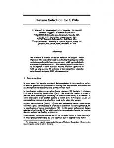
Figure 1. In boosting-based vision applications, the rectangular features/weak classifiers need to be updated due to varying appearance and shape of the object. This paper proposes a gradient-based approach to efficiently perform feature updating.
It is the seminal work of Viola and his colleagues [21,23] that bridges the gap of weak classifier design in boosting and the feature selection step, a critical component in any vision application. The introduced integral image [23] brings the fast computations of visual features, enabling the possibility of performing exhaustive search over a very large feature (hypothesis) space. Such an exhaustive feature selection might be fine for offline learning tasks. However, it becomes a less satisfactory option for online applications, such as object tracking [2,9], where an adaptive method is needed to continuously update the existing classifiers to handle the appearance/shape variations of the object over time. With the real-time constraint, the exhaustive feature selection over a very large hypothesis space is obviously prohibited. To remedy this problem, Grabner and Bischof [8] propose a novel feature selection method, where a batch of selectors are constructed to take a random guess selection of the features. It might be effective to eventually pick up the discriminative features, this random selection, however, is still far from efficiency. It does not fully take advantage of the nature that for online applications, such as object tracking, the sequential data consumed by the online algorithm usually shows very high correlation over time, while the random selection in [8] does not really capture this time dependency. To better exploit the correlation of sequential data, as shown in the notional example of Figure 1, this paper pro-
poses a gradient-based feature selection approach for online boosting. Assuming a feature set generally trained from offline data is available, and during online learning newly labeled samples are sequentially given, our approach iteratively updates each feature using the gradient descent method. Formulated into the GentleBoost framework [7], the gradient-based feature selection proceeds by continuously minimizing the weighted least square error between the estimated feature response and its true label. When integrated into the online boosting, the proposed approach presents a unified objective for both feature selection and weak classifier updating. As shown in Figure 1, the three colorized rectangular features get updated by minimizing the objective in a gradient descent sense. Our scientific findings and contributions can be summarized as follows: ¦ We propose a novel non-exhaustive feature selection approach based on the gradient descent method. This is a much more efficient scheme of learning discriminative features compared to the common way of searching the feature hypothesis space exhaustively. ¦ We present an online boosting algorithm by integrating this gradient-based feature selection with the GentleBoost framework. It leads to a unified objective for both feature selection and weak classifier updating. ¦ We pick two popular applications to demonstrate the effectiveness and efficiency of the proposed approach, i.e., online learning of person detector and discriminative tracking of walking person. The quantitative analysis and comparison highlight the advantage of our proposal compared to the offline boosting and previous online boosting methods.
2. Related Work As a general machine learning algorithm, boosting is well known for several nice properties, such as simple implementation, good generalization to unseen data, and robustness to outliers [16]. Considerable progress has also been made on applying boosting to various computer vision problems, such as image retrieval [21], face detection [24], person detection [11,25], object tracking [2,9], image alignment [15], etc. During boosting learning, how to efficiently select features is an important issue, especially critical to vision applications. To avoid the costly exhaustive feature selection, Treptow and Zell [22] propose a random feature search method via evolutionary algorithm. Dollar et al. [5] recently present a notion of feature selection using gradient descent. In above applications, boosting mainly serves as an offline learning machine, i.e., once learned from training data, the boosted classifier is fixed during testing. Recently, research interests are also raised to apply learning methods to online vision applications [2, 3, 9, 10, 14, 17, 18]. For example, in object detection, Nair et al. [17] and Javed et al. [10] utilize a co-training approach to classify
each incoming data and use it in incrementally online updating of the object classifier. In object tracking, Collins et al. [3] and Lim et al. [14] continuously update the appearance trackers through online discriminant learning. Boosting algorithms have also been applied to online vision. Avidan [2] proposes to combine an ensemble of weak classifiers into a strong classifier using AdaBoost to handle object appearance variations, though their classifier updating is still treated in an offline learning mode. Online applications deal with sequential data, thus require the capability of weak classifiers updated in an online fashion. Oza and Russell [19] make the primary efforts on studying the sequential learning of boosted classifiers, called online boosting. They prove that with the same training set, online boosting converges statistically to offline one as the number of iterations goes to infinity. Based on [19], Grabner and Bischof [8, 9] propose a novel online boosting framework, which we refer by “OB”, and apply it to vision applications. Our online boosting differs from OB in that a gradientbased approach is proposed to perform feature selection and weak classifier updating given the sequential data. Detailed comparisons between these two methods are presented in later sections. Our work also advances the gradient-based feature selection notion of Dollar et al. [5] by providing the explicit formula of gradient-based updating.
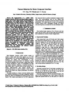
3. Offline Boosting We start with the introduction of the conventional boosting in the offline training mode, which we refer by “offline boosting” (OFB). Boosting-based learning iteratively selects weak classifiers PMto form a strong classifier using summation: F (x) = m=1 fm (x), where F (x) is the strong classifier and fm (x) is the weak classifier. There are different variants of boosting proposed in the literature [16]. We use the GentleBoost algorithm [7] based on two considerations. First, unlike the commonly used AdaBoost algorithm [6], the weak classifier in the GentleBoost algorithm is a soft-decision classifier with continuous output. This enables the strong classifier’s score to be smoother and favorable for computing derivatives. In contrast, the hard weak classifiers in the AdaBoost algorithm lead to a piecewise constant strong classifier that is difficult to optimize. Second, as shown in [13], for object detection tasks, the GentleBoost algorithm outperforms other boosting methods in that it is more robust to noisy data and more resistant to outliers. Algorithm 1 summarizes the GentleBoost algorithm. To apply it to vision applications, we firstly define the weak classifier. Given the recent success of Histogram of Oriented Gradient (HOG) feature in object detection [4, 12], we adopt it in our weak classifier design and evaluate HOG by integral histogram computation [20]. As shown in Figure 2(a), the HOG can be parameterized by (x0 , y0 , x1 , y1 ), where (x0 , y0 ) and (x1 , y1 ) are the two corners of a cell. To
Input: Training data {xi ; i ∈ [1, K]} and their corresponding class labels {yi ; i ∈ [1, K]}. Output: A strong classifier F (x). 1. Initialize weights wi = 1/K, and F (x) = 0. 2. for m = 1, 2, ..., M do (a) Fit the regression function fm (x) by weighted least square of yi to xi with weightsP wi 2 fm (x) = argminf ∈F ²(f ) = K i=1 wi (f (xi ) − yi ) . (b) Update F (x) = F (x) + fm (x). (c) Update the weights by wi = P wi e−yi fm (xi ) and normalize the weights such that K i=1 wi = 1. end P 3. Output the classifier sign[F (x)] = sign[ M m=1 fm (x)].
Algorithm 1: The GentleBoost algorithm.
where β is the LDA projection direction, t is the threshold and p are the parameters of the weak classifier p = [x0 , y0 , x1 , y1 , β, t]T . Given a cell location (x0 , y0 , x1 , y1 ), the histogram features h are computed from all training data via the integral histogram. Weighted LDA is applied to compute β, and finally t is obtained through binary search along the span of LDA projections of all training data, such that the weighted least square error (WLSE) is minimal. Similar to [15], we use the atan() function in the weak classifier, instead of the commonly used decision stump, because of its derivability with respect to the parameters p.
4. Gradient Feature Selection 4.1. Problem definition
(a)
(b)
(c) 0.08
We define the feature selection as a process of updating the parameters of each weak classifier pm . As shown in Step 2(a) of Algorithm 1, the WLSE is used in selecting the weak classifier from the hypothesis space during the boosting iteration. Hence, it is natural to use the WLSE as the objective function for the feature selection (updating). This leads to the following problem we are trying to solve
0.06 0.04 0.02 0
(d)
10
20
30
Figure 2. (a) The parametrization of a cell; (b) The gradient map; (c) The HOG of a block; (d) The HOG features of positive and negative samples.
incorporate spatial information into HOG, a 2 × 2 cell array is used to form a block. For each cell, the b-bin histogram of the gradient magnitude at each orientation is computed. The concatenation of the HOG for 4 cells within one block forms a 4b-dimensional vector, as shown in Figure 2(c). The large hypothesis space F, where (x0 , y0 , x1 , y1 ) resides, is obtained via an exhaustive construction within the template coordinate system. For example, there are more than 300, 000 such block features for a template with the size of 30 × 30. Hence, the exhaustive feature selection process, Step 2(a) in Algorithm 1, is the most computationally intensive step in the GentleBoost algorithm. When a multi-dimensional feature vector, such as the histogram, is used in the weak classifier, the conventional method of computing the threshold in the decision stump classifier, which often works comfortably with a 1-D feature, can not be directly applied. In this paper, we employ the idea of boosted histogram proposed by Laptev [11]. As shown in Figure 2(d), a weighted Linear Discriminative Analysis (LDA) is applied to the histogram features of positive and negative samples, and results in the optimal projection direction β. Thus, all histograms can be converted to 1-D features by computing the inner product with β. In summary, we use the following weak classifier: f (x; p) =
2 atan(β T h(x0 , y0 , x1 , y1 ) − t), π
(1)
min ²(f (x; p)) = min p
p
K X
wi (f (xi ; p) − yi )2 .
(2)
i=1
In the context of feature selection, solving this problem means that given the initial parameters p(0) , we look for the new parameters of the weak classifier that can lead to smaller WLSE on the dataset {xi } with K samples in total. We choose to use the gradient descent method to solve this problem iteratively.
4.2. Algorithm derivation Plugging Eq. 1 into Eq. 2, the function to be minimized is ²=
K X
2 wi ( atan(β T hi (x0 , y0 , x1 , y1 ) − t) − yi )2 . (3) π i=1
Taking the derivative with respect to p gives K
X d² dfi = 2wi (f (xi ) − yi ) , dp dp i=1 where have
dfi dp
(4)
∂fi ∂fi ∂fi ∂fi ∂fi ∂fi T = [ ∂x ] . Based on Eq. 1, we 0 ∂y0 ∂x1 ∂y1 ∂β ∂t
i β T ∂h ∂fi 2 ∂z = , z = x0 , y0 , x1 , y1 , ∂z π 1 + (β T hi − t)2 2 hi ∂fi = , ∂β π 1 + (β T hi − t)2 ∂fi 2 −1 = . T ∂t π 1 + (β hi − t)2
(5)
As an example, we show how to compute the derivative of the histogram feature with respect to one of the cell ∂hi . The remaining partial location parameters x0 , i.e., ∂x 0 ∂hi ∂hi ∂hi derivatives, ∂x1 , ∂y0 and ∂y1 , can be computed similarly. As mentioned in Section 3, hi is a 4b-dimensional vector hi (x0 , y0 , x1 , y1 ) = [hi,1 , hi,2 , · · · , hi,4b ]T computed from the 4 cells of a block. Given a labeled image xi , the gradient map is computed and a set of integral images of the magnitude of the gradient at each orientation {¯ xi,1 , x ¯i,2 , · · · , x ¯i,b } is obtained. Since all 9 corners of the 2 × 2 cells can be fully described by the cell location (x0 , y0 , x1 , y1 ), each bin of the histogram can be computed via accessing the integral image x ¯i,j at the corresponding pixel location defined as follows hi,j = x ¯i,j (x0 , y0 ) + x ¯i,j (x1 , y1 ) − x ¯i,j (x0 , y1 ) −¯ xi,j (x1 , y0 ), hi,j+b = x ¯i,j (x1 , y0 ) + x ¯i,j (2x1 − x0 , y1 ) − x ¯i,j (x1 , y1 ) −¯ xi,j (2x1 − x0 , y0 ), hi,j+2b = x ¯i,j (x0 , y1 ) + x ¯i,j (x1 , 2y1 − y0 ) − x ¯i,j (x1 , y1 ) −¯ xi,j (x0 , 2y1 − y0 ), hi,j+3b = −¯ xi,j (2x1 − x0 , y1 ) − x ¯i,j (x1 , 2y1 − y0 ) +¯ xi,j (x1 , y1 ) + x ¯i,j (2x1 − x0 , 2y1 − y0 ). (6) where i ∈ [1, K] and j ∈ [1, b]. The Eq. 6 defines total 4b equations to compute the 4b-dimensional orientation histogram hi . Given above hi definition, the derivative of hi with respect to x0 can be computed by ∂¯ xi,j ∂¯ xi,j ∂hi,j = |(x0 ,y0 ) − |(x0 ,y1 ) , ∂x0 ∂x ∂x ∂hi,j+b ∂¯ xi,j ∂¯ xi,j =− |(2x1 −x0 ,y1 ) + |(2x1 −x0 ,y0 ) , ∂x0 ∂x ∂x ∂hi,j+2b ∂¯ xi,j ∂¯ xi,j = |(x0 ,y1 ) − |(x0 ,2y1 −y0 ) , ∂x0 ∂x ∂x ∂¯ xi,j ∂¯ xi,j ∂hi,j+3b = |(2x1 −x0 ,y1 ) − |(2x1 −x0 ,2y1 −y0 ) , ∂x0 ∂x ∂x (7) ∂¯ x
where ∂xi,j |(x0 ,y0 ) is the partial derivative of x ¯i,j with respect to the horizontal axe x and evaluated at (x0 , y0 ), and can be easily computed via discrete differentiation such as ∂¯ xi,j 1 xi,j (x0 + 1, y0 ) − x ¯i,j (x0 − 1, y0 )]. ∂x |(x0 ,y0 ) = 2 [¯ Please note that the above feature gradient derivations are not necessarily only suitable to the HOG feature. In fact, all integral-image-enabled features can have similar formulas to compute the gradients, thus can all be used in the proposed framework.
5. Online Boosting 5.1. Online boosting with gradient feature selection Understanding that feature gradients, such as ∂hi ∂hi ∂hi ∂hi [ ∂x , , , ∂y1 ], bring the connection between 0 ∂x1 ∂y0
Input: Training data {xi ; i ∈ [1, K]}, their corresponding class labels {yi ; i ∈ [1, K]}, and an initial set of weak classifiers {fm (pm ); m ∈ [1, M ]}. Output: An updated strong classifier F (x). 1. Initialize weights wi = 1/K, and F (x) = 0. 2. for m = 1, 2, ..., M do d² |pm using Eq. 3 and Eq. 4. (a) Compute ²(pm ) and dp (b) if ²(pm ) is decreasing then d² Update pm = pm − dp |pm . Jump to (a). end (c) Update F (x) = F (x) + fm (x; pm ). (d) Update the weights by wi = P wi e−yi fm (xi ) and normalize the weights such that K i=1 wi = 1. end 3. Output the classifier P sign[F (x)] = sign[ M m=1 fm (x; pm )].
Algorithm 2: The proposed gradient-based online boost algorithm (GOB). minimizing the WLSE of the weak classifier and feature updating, now we introduce our online boosting algorithm. Our online boosting follows the basic scheme of the conventional offline boosting. That is, weak classifier selection and weights updates are performed in each iteration of the boosting. However, these two approaches differ in the weak classifier selection step. In the offline boosting, this step is achieved by exhaustively evaluating all classifier candidates in a hypothesis space, which is often huge due to the over-complete feature set. Hence, this is a very computationally demanding operation. In contrast, our online boosting treats the weak classifier selection as a gradient descent optimization problem. Our approach takes an initial set of weak classifiers and a number of labeled training samples as inputs. For each weak classifier fm (pm ), the online boosting iteratively updates the feature parameters pm according to the above computed gradient d² dp . The objective function ²(pm ) is computed at each iteration and expected to keep decreasing. The iteration will cease if the objective arrives at a minimum, or the d² magnitude of the gradient | dp | is smaller than a threshold. Algorithm 2 summarizes our algorithm, which we refer as “Gradient-based Online Boosting” (GOB).
5.2. Comparison between OB and GOB We briefly describe the conventional OB [8] in Algorithm 3, in order to compare it with the proposed GOB. In OB, the strong boosted classifier is composed of a batch of selectors, and each selector contains a random subset of weak classifiers. During the updating, given a new training sample, each selector is responsible for selecting the best weak classifier from its subset, by updating all classifiers in its subset simultaneously and choosing the one with the
for each selector do (a) for each weak classifier in the selector do Update the weak classifier and compute error. end (b) Choose the weak classifier with lowest error. (c) Update sample importance weights. (c) Replace the worst weak classifier with a randomly selected feature. end
Algorithm 3: The simplified description of the conventional online boost algorithm (OB).
lowest error. All selectors will conduct the same updating sequentially. Note that, unlike GOB that both the feature (block location) and the weak classifier (LDA direction and threshold) get updated, OB only updates the weak classifier (threshold) [8]. The selector will also update its feature set by replacing the worst weak classifier in its subset with a randomly selected feature. OB depends on random selections of the discriminative features, which may show good performance when the object being tracked is rigid, and camouflage features are around. However, this method might suffer from the large object deformation. Once object deformation appears, most of the local rectangular/block features may become invalid due to the local mis-alignment. This consequently will result in OB continuously looking for new features to add into the selector. However, such a process is blindly random without considering the nature that a local deformation strongly implies that a local shifting of the originally found rectangular feature is still very likely to be a good discriminative feature. In essence, the proposed gradientbased feature selection method is to train each rectangular feature doing exactly this local object deformation tracking in a discriminative sense. Therefore, the overall capacity of our algorithm to handle the object deformation is much better than OB, which we will demonstrate in Section 6.2. We can also compare the computational costs of OB and GOB to see the efficiency of our method. Assuming M weak classifiers (GOB) or selectors (OB) are trained in total, each one of the M selector has N weak classifiers and the cost of updating each weak classifier is C, the average cost of updating all weak classifiers is O(N CM ) for OB. Similarly, in our proposal, assuming the average number of iterations for updating one weak classifier is n, the cost of updating all weak classifiers is O(nCM ). For OB, it is reported that N = 250 [8]. However, we experimentally learn that n = 2. Thus, a huge computational gain is observed using our approach. [8] also mentions an efficient version of the algorithm by using the same N weak classifiers for all selectors. Hence, the computation cost will reduce to O(N C + M ) where our algorithm is still more efficient than OB in this case.
Figure 3. Positive samples of the person detection database.
6. Experiments We demonstrate the proposed gradient-based online boosting idea with two popular applications: person detection and person tracking.
6.1. Person detection Person detection is often achieved by learning a dedicated classification-based detector from labeled data. Given large amount of positive training samples and infinite number of negative samples in theory, the computation and storage burden can make the training impractical, especially when new samples are received sequentially and detector updating is needed. There are three ways to handle this issue via boosting. First, if the computation and storage allow, we can re-train the detector with all available data using OFB. Second, when the computation burden exceeds the limit, we can test the detector on all available data first, and only re-train on a challenging subset of the original data. We call this approach as “Offline Selective Boosting” (OFSB). Third, GOB can be used to update the detector with the newly received samples. We use a labeled person database with 915 positive and 6361 negative samples. Some of the typical samples are shown in Figure 3. To imitate the real-world scenario of continuously receiving new data in sequential learning, we partition this database into three distinct sets: the training set s1 , the updating set s2 , and the test set s3 , where each has 52 , 52 , and 15 positive and negative samples of the database. Furthermore, s2 is evenly partitioned into 6 subsets, {s2,1 , · · · , s2,6 }, which are assumed to arrive sequentially. Figure 4 illustrates our experimental design. To begin the experiments, an initial classifier is trained from s1 using OFB. When a new data set arrives, such as s2,1 or s2,2 , OFB is re-trained on all available data up to the current time. However, when s2,3 arrives, it is assumed that re-training on all data starts to become impractical due to the demanding computation cost and memory requirement. Hence, OFSB is used in this case, and the present classifier is tested on the set of {s1 , s2,1 , s2,2 , s2,3 }. The sample, which is closer to the classification boundary (measured by the strong classifier response), is added into a subset, until the size of this subset reaches the allowed limit, i.e., the size of {s1 , s2,1 , s2,2 }. Finally, offline boosting is used to re-train a classifier based on this chosen subset. In contrast, when each subset of s2 sequentially arrives, we can also use
s1
s2
s3 Test
OFB Test OFSB Test GOB
0
1
2
3
4
5
6
Figure 4. Experimental design. Three learning schemes, offline boosting (OFB), offline selective boosting (OFSB) and gradientbased online boosting (GOB), are used to train and update a detector from s1 and s2 . After each update, s3 is used to test the detection performance.
True Detection Rate
10
10
10
10
0
-0.01
OFB - FAR=0.1 OFB - FAR=0.05 OFB - FAR=0.01 OFB - FAR=0.005 GOB - FAR=0.1 GOB - FAR=0.05 GOB - FAR=0.01 GOB - FAR=0.005
-0.02
-0.03
0
1
2
3 4 Ne w Datas et Index
5
6
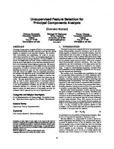
Figure 5. Detection performance of continuously learned boosted classifier from new data sets. The horizontal axis represents the index of the new data set while the vertical axis represents the detection rate of the updated classifier tested on s3 . Stable and increasing performance can be observed from our gradient-based online boosting (GOB) algorithm. 1
2
(a) 4
0.5
6 10
20
30
40
50
60
70
80
90
100
0 x 10
2
-3
5
(b) 4 6 10
20
30
40
50
60
70
80
90
100
0 5
2
(c) 4 6 10
20
30
40
50
60
70
80
90
100
0
Figure 6. Updating of the weak classifiers in GOB. The vertical axes is the new data set index, from 1 to 6. The horizontal axes is the index of weak classifier. The brightness of each grid indicates the amount of changes for the parameter of each weak classifier. (a) MSE of the box location change; (b) Angle change of the LDA projection; (c) Change of the threshold.
GOB to continuously update the present classifier based on the new subset only. After each re-training or updating, the performance of the resulting boosted classifier is tested on s3 , as shown in Figure 5. For clear illustration purpose, the detection ratefalse alarm curve is not shown. Instead we sample the curve at four particular false alarm rates (FAR), namely 0.1, 0.05, 0.01, 0.005. Note that the dash line represents OFB when the new data set index is less than 3. Otherwise, it is OFSB. Figure 6 shows the amount of changes in the weak classifiers during GOB learning. It can be seen that majority of
the weak classifiers actually being updated when receiving new data. A number of observations can be made. First, as expected, overall both online and offline boosting increase their performance as taking more data for training. Second, since the re-training process of OFB/OFSB throws away previously trained classifier, it is more likely to obtain a classifier that has unstable performance. While GOB always starts with the prior knowledge, i.e., the present classifier, to improve its capacity on the new data, meanwhile still maintain its discriminative power on the old data. Hence, the online boosting demonstrates a stable and increasing performance on the unseen data set s3 . GOB also has a huge computational advantage over OFB/OFSB. For the experiments in Figure 5, GOB takes around 15 minutes to finish updating when receiving each new data set. However, OFB/OFSB take more than 7 hours to finish re-training once. Both time costs are based on a MatlabTM implementation and exclude the computation of feature extraction (computing integral images of oriented gradients).
6.2. Person tracking Following the same weak classifier design as in person detection, the proposed GOB is also applied to person tracking application. The main idea of applying online boosting in this domain is to formulate the tracking problem as a discriminative training process, which continuously updates the boosted classifier to discriminate the human region from its nearby backgrounds. We take a similar tracking-and-updating process cycle as [8]. Once an optimal human region is tracked with the previously trained boosted classifier, a set of new training data is cropped from this location (positive data) and nearby neighborhoods (negative data). The weak classifiers are updated with this new data set. Essentially, a boosted classifier trained in this way manages to learn a drifting detector of the tracker. As long as the tracker keeps following the person with accurate alignments, the drifting detector will report higher classification scores; on the contrary, if the tracker deviates from its optimal location, negative responses will be returned. One example of applying the proposed GOB algorithm to person tracking in surveillance videos is shown in Figure 7(a), where as the person walks towards the camera, his body pose also gradually changes from a side view to the front view. GOB is capable of learning to follow this turning action, and continuously track the person. The colorized small rectangles illustrate the weak classifiers that have changed their box location parameters (x0 , y0 , x1 , y1 ) by GOB at the corresponding frame. Due to the balance between the classification performance and efficiency, we select 50 weak classifiers in total for all tracking experiments.
Figure 7. Tracking results by the proposed GOB algorithm. (a) a person changing pose; (b) a person under severe occlusion and continuously turning over; (c) a person making a full turn.
S trong Clas s ifie r S c ore
5
(a)
(b) 10
2.5 20
8
0
-5
60
1 100
2
Offline boos ting 0
20
40
1.5
80
4
Gra dient ba s ed online boos ting -10
2
40
6
0.5
120
60 80 Frame Index
100
120
140
Figure 8. Strong classifier scores (GOB vs OFB) evaluated at the optimal location returned by GOB.
Without surprise, an offline trained frontal view person classifier can not reliably track the subject, and loses tracking at the very early stage of the sequence. From Figure 8, it is easy to see the benefits of online classifier updating. The strong classifier responses with the gradient updating are much higher than the one without updating. It verifies the power of the gradient-based boosting to keep learning better discriminant features (weak classifiers) to separate the person from backgrounds. The proposed GOB framework is particularly suitable for the tracking application, since, during the successive frames, the object of interest will generally only show minor changes in terms of appearance and shape. These minor but non-ignorable changes could be best captured by the gradient learning framework. During the updating within two continuous frames, most of the weak classifiers will not change their feature locations, reflecting the fact that the object parts corresponding to these feature locations show no difference between two frames, while only a few feature locations will get updated, implying those regions are undergoing local shape deformation and/or appearance change. This property is demonstrated in Figure 7(a), where the number of colorized rectangles (weak classifiers with changed locations) only represents a small portion of total weak classifiers (50) we applied to the sequence. Further-
0 0
20
40
60 80 Frame Index
100
120
140
0 10 20 30 40 50 Weak Classifier Index
Figure 9. (a) The number of weak classifiers that change their feature box locations over time. Higher number indicates relative larger shape and appearance deformation; (b) MSE of the box location changes over time. The intensity reflects the magnitude of the feature location changes.
more, in Figure 9(a), we show the plot of the number of weak classifiers with changed locations through updating for the sequence in Figure 7(a). It is observed that during the whole sequence at most one-fifth (10/50) of the weak classifiers update their locations between successive frames. It validates that GOB is very efficient, yet still effective to capture the minor appearance changes using discriminative training. Also, the higher number of updating indicates relative larger shape and appearance deformation. In Figure 9(b), we illustrate a similar figure as in Figure 6(a), while here the updating is for online tracking application. Again, the relative less updating reflects the fact that the unseen new data received over time is actually showing strong correlations with the previous ones. Hence, only minor updating is needed, which is particularly true for tracking application. In Figure 7(b), we show a challenging sequence that our GOB can tackle. The object being tracked is under very severe occlusion, when a girl wearing the white clothes is approaching and passing the object of interest. GOB shows great performance on learning the relatively stable yet dis-
Sequence ID Conventional online boosting (OB) Gradient-based online boosting (GOB)
1 15.1 6.2
2 Lost 10.9
3 14.1 7.1
4 Lost Lost
5 Lost 7.7
6 Lost 11.0
7 5.0 5.5
8 Lost 5.4
9 4.6 4.4
10 Lost 8.8
Table 1. Average tracking errors of two online boosting-based trackers. The average size of the tracking window is 140 × 46 pixels.
criminant features (the head and shoulder in this example), thus managing to follow the person even under such a challenging situation. Figure 7(c) is another example where the person makes a full turn and walks back. Finally, we also carry out a quantitative study on tracking using two methods: the GOB tracker and the OB tracker [8,9]. We strictly follow the OB algorithm presented in [8] to repeat their implementation, where each selector has a different subset of the weak classifiers. We test on ten video sequences (4000+ frames in total) from the CAVIAR database [1]. The ground truth locations of these data are given. The average tracking errors against the ground truths are reported in Table 1. The tracking error is defined as the pixel distance between the center of the bounding box returned by the trackers and that of the ground truth. Consistent with the discussion in Section 5.2, our GOB tracker outperforms the OB tracker. The gained performance is attributed to the local gradient search capability in each weak classifier updating, so as to keep following its discriminative yet shifted/deformed features.
7. Conclusions We have introduced a novel gradient-based feature selection approach for online boosting. Assuming a generally trained feature set and labeled samples are given, our approach iteratively updates each feature using the gradient descent method, by minimizing the weighted least square error between the estimated feature response and the true label. Furthermore, we integrate the gradient-based feature selection with an online boosting framework. The proposed online boosting is applied to the person detection and tracking applications. Extensive experiments demonstrate the effectiveness and efficiency of our proposal. Future directions of this work include extending online learning for other variants of boosting and applying online boosting into other vision applications.
Acknowledgement This project was supported by awards #2005-IJ-CX-K060 and #2006-IJ-CX-K045 awarded by the National Institute of Justice, Office of Justice Programs, US Department of Justice. The opinions, findings, and conclusions or recommendations expressed in this publication are those of the authors and do not necessarily reflect the views of the Department of Justice.
References [1] http://homepages.inf.ed.ac.uk/rbf/CAVIAR/. [2] S. Avidan. Ensemble tracking. IEEE Trans. on Pattern Analysis and Machine Intelligence, 29(2):261–271, 2007. [3] R. Collins, Y. Liu, and M. Leordeanu. On-line selection of discriminative tracking features. IEEE Transaction on Pattern Analysis and Machine Intelligence, 27(10):1631–1643, 2005. [4] N. Dalal and W. Triggs. Histograms of oriented gradients for human detection. In Proc. IEEE Computer Vision and Pattern Recognition, San Diego, California, volume 1, pages 886–893, 2005. [5] P. Dollar, Z. Tu, H. Tao, and S. Belongie. Feature mining for image classification. In Proc. IEEE Computer Vision and Pattern Recognition, Minneapolis, Minnesota, 2007. [6] Y. Freund and R. Schapire. A decision-theoretic generalization of on-line learning and an application to boosting. Journal of Computer and System Sciences, 55(1):119–139, 1997. [7] J. Friedman, T. Hastie, and R. Tibshirani. Additive logistic regression: A statistical view of boosting. The Annals of Statistics, 38(2):337–374, 2000. [8] H. Grabner and H. Bischof. On-line boosting and vision. In Proc. IEEE Computer Vision and Pattern Recognition, New York, NY, volume 1, pages 260–267, 2006. [9] H. Grabner, M. Grabner, and H. Bischof. Real-time tracking via on-line boosting. In Proc. 17th British Machine Vision Conference, Edinburgh, UK, volume 1, pages 47–56, 2006. [10] O. Javed, S. Ali, and M. Shah. Online detection and classification of moving objects using progressively improving detectors. In Proc. IEEE Computer Vision and Pattern Recognition, San Diego, California, volume 1, pages 696–701, 2005. [11] I. Laptev. Improvements of object detection using boosted histograms. In Proc. 17th British Machine Vision Conference, Edinburgh, UK, volume 3, pages 949– 958, 2006. [12] K. Levi and Y. Weiss. Learning object detection from a small number of examples: The importance of good features. In Proc. IEEE Computer Vision and Pattern Recognition, Washington, DC, volume 2, pages 53–60, 2004. [13] R. Lienhart, A. Kuranov, and V. Pisarevsky. Empirical analysis of detection cascades of boosted classifiers for rapid object detection. In Proc. 25th Pattern Recognition Symposium, Madgeburg, Germany, pages 297–304, 2003. [14] J. Lim, D. A. Ross, R.-S. Lin, and M.-H. Yang. Incremental learning for visual tracking. In Advances in Neural Information Processing Systems 17, NIPS, Vancouver, Canada, pages 793–800, 2004. [15] X. Liu. Generic face alignment using boosted appearance model. In Proc. IEEE Computer Vision and Pattern Recognition, Minneapolis, Minnesota, 2007. [16] R. Meir and G. Raetsch. An introduction to boosting and leveraging. S. Mendelson and A. Smola, Editors, Advanced Lectures on Machine Learning, LNAI 2600. Springer, 2003. [17] V. Nair and J. Clark. An unsupervised, online learning framework for moving object detection. In Proc. IEEE Computer Vision and Pattern Recognition, Washington, DC, volume 2, pages 317–324, 2002. [18] A. Opelt, M. Fussenegger, A. Pinz, and P. Auer. Weak hypotheses and boosting for generic object detection and recognition. In Proc. 8th European Conf. Computer Vision, Prague, Czech Republic, volume 2, pages 71–84, 2004. [19] N. Oza and S. Russell. Experimental comparisons of online and batch versions of bagging and boosting. In Proc. 7th ACM SIGKDD International Conference on Knowledge Discovery and Data Mining, pages 359–364, 2001. [20] F. Porikli. Integral histogram: A fast way to extract histograms in cartesian spaces. In Proc. IEEE Computer Vision and Pattern Recognition, San Diego, California, volume 1, pages 829–836, 2005. [21] K. Tieu and P. Viola. Boosting image retrieval. Int. J. Computer Vision, 56(12):17–36, 2004. [22] A. Treptow and A. Zell. Combining adaboost learning and evolutionary search to select features for real-time object detection. In IEEE Congress on Evolutionary Computation, volume 2, pages 2107–2113, 2004. [23] P. Viola and M. Jones. Rapid object detection using a boosted cascade of simple features. In Proc. IEEE Computer Vision and Pattern Recognition, Hawaii, volume 1, pages 511–518, 2001. [24] P. Viola and M. Jones. Robust real-time face detection. Int. J. Computer Vision, 57(2):137–154, 2004. [25] P. Viola, M. Jones, and D. Snow. Detecting pedestrians using patterns of motion and appearance. Int. J. Computer Vision, 63(2):153–161, 2005.