(Grenander et. al. [9]). In situations where the rank is ..... [13] Anuj Srivastava, Michael Miller, and Ulf Grenander. Ergodic Algorithms on Special Euclidean ...
Gradient Flows on Projection Matrices For Subspace Estimation Anuj Srivastava
�
Daniel R. Fuhrmann y
Keywords: gradient flows, Grassman manifold, sensor array processing, subspace estimation
an observed time series. Similarly in computer vision applications, such as robotic control or automated navigation, the observations are generated from projective transformation of the three-dimensional scene elements onto the focal plane of the camera. The loss of scale (or range) information results in the directional data and hence the knowledge is restricted to (real) projective spaces. As described in Bucy [4], Smith [11], Fuhrmann et. al. [7], and many others, such problems are naturally posed on Grassmanian manifolds, the space of lower-dimensional subspaces of some larger Euclidean space. Even though they provide a natural domain to pose optimization problems, the use of conventional techniques on these manifolds is limited. The fundamental issue is that they have curved geometry, i.e. they are not vector spaces. Gradient calculus behind the usual optimization techniques needs to be modified to account for the curved geometry. For Euclidean parameterizations, or parameterizations restricted to unit spheres, gradient and stochastic gradient techniques have been applied earlier, including Pisarenko’s harmonic retrieval approach to finding eigen-decomposition of a given matrix. We propose a more general approach to find the optimal points of a bigger class of cost functions. It is a gradientbased optimization technique which accounts for the curved geometry of such manifold representations and generates global solutions, if they exist. The cost functions can come, for example, from maximum-likelihood or a Bayesian aposteriori formulation or a filtering formulation. We have derived a similar technique for Bayesian optimization in Srivastava [12] but restricted to Lie groups and hence not applicable to all differentiable manifolds. There are essentially two new aspects to this approach:
Abstract Estimation of dynamic subspaces is important in blindchannel identification for multiuser wireless communications and active computer vision. Mathematically, a subspace can either be parameterized non-uniquely by a linearly-independent basis, or uniquely, by a projection matrix. We present a stochastic gradient technique for optimization on projective representations of subspaces. This technique is intrinsic, i.e. it utilizes the geometry of underlying parameter space (Grassman manifold) and constructs gradient flows on the manifold for local optimization. Addition of a stochastic component to the search process guarantees global minima and a discrete jump component allows for uncertainty in rank of the subspace (simultaneous model order estimation).
1 Introduction A variety of engineering problems involve inferences on low-dimensional subspaces associated with some larger observation spaces. As for example, in signal estimation using an antenna array, the signal subspace of the sample covariance matrix provides information about the directional location of the signal transmitters. Therefore, estimation of signal subspaces plays an important role in emerging techniques for blind channel identification in multiuser wireless communication systems (see for example [10, 1, 14]). The base station receivers must adaptively determine the response vector for each of many users, transmitting simultaneously over a wide-band channel, without the use of special training sequences. Comon & Golub [5] compare a variety of techniques used in tracking low-dimensional range subspaces associated with changing sample covariance of
1. Representation by projection matrices: Let Vn;m be the space of all n � m (n > m) orthogonal matrices and Om be the space of m � m orthogonal matrices. The quotient space Vn;m =Om , is called the Grassmanian manifold Gn;m ; it is the set of all m-dimensional subspaces of IRn . An element of Gn;m can be represented by any set of m, linearly independent n-vectors which span that subspace. An alternative is to represent a subspace by a size n � n, rank m projection matrix. Representation of subspaces using projection
� Department of Statistics, Florida State University, Tallahassee, FL 32306 y Department of Electrical Engineering, Washington University, St. Louis, MO 63130
1
there exists a neighborhood U and a map � : U 7! IRJ , such that � is diffeomorphic between U and �(U ). For the exponential representation � is given by
matrices, which was proposed in Fuhrmann et al. [7], is attractive due to the uniqueness of representation. To illustrate uniqueness, consider the following: a plane in IR3 can be represented by any pair of linearly independent 3-vectors which span it. There is an infinite number of pairs which can be used, but if we consider a projection matrix on to the plane, it is unique and can be used to identify the plane completely. If v 2 IR3 is the unit vector normal to the plane then P = (I ? v � v y) is the projection matrix.
�?1 (A) = e?A � Im � eA (1) where A is a n � n skew-symmetric matrix and Im is a n � n diagonal matrix with only m entries 1 and rest zeros. Notice that in A only J elements need to be specified and they form a local representation of the point e?A � Im � eA 2 IP .
2. Intrinsic optimization techniques: Our approach is intrinsic, in that, we will use the geometry of underlying space to construct an optimization process which stays in that space. Similar philosophy has also been advocated in Smith [11] to solve a variety of filtering problems on such manifolds. The extrinsic approaches, embed the parameter space in a higher-dimensional Euclidean spaces, and solve a constrained optimization problem in the bigger space. Using the underlying geometric structure, wherever possible, will provide insight into the physical interpretation of the solutions and, perhaps, improve the estimation process. Furthermore, we seek to develop stochastic gradient techniques along the lines of simulated annealing (Geman et. al. [8]) or diffusion sampling (Grenander et. al. [9]). In situations where the rank is unknown addition of discrete moves to accommodate the variability in unknown subspace dimensions via jumps will lead to a Jump-Diffusion analysis ([12]).
1. Tangent Structure: Tangents determine the directional derivatives and the gradient vectors. Define a family of differentiable, one-parameter curves on the manifold passing through a point P 2 IP and identify all the curves which result in the same derivative (with respect to that parameter). Each equivalent class is represented by a derivative vector, also called the tangent vector (even though it is actually an n � n matrix), and the resulting set of equivalent classes forms the tangent space at that point (please refer to [2, 6] for details). It should be noted that the tangent spaces are always vector spaces, that is, they have flat geometry. Let TP (IP ) denote be the J -dimensional space of vectors tangent to IP at point P . For any n � n skew-symmetric matrix A, the matrix
There are two basic questions which need to be answered: (i) how to evaluate derivatives of functions on IP ?, and (ii) how to construct processes taking values in IP ? The answers come from study of following two components:
Y =A�P ?P �A (2) is tangent to IP at P 2 IP . The inner product on
We start with a brief review of the underlying geometry.
2 Geometry of Projection Matrices
the tangent space (Riemannian metric) is given by hhY1 ; Y2 ii = trace(Y1�Y2T ). The relationship between the tangent vectors and the skew-symmetric matrices is not one-to-one, i.e. many skew-symmetric A can result in the same tangent element Y . Associated with an element Y 2 TP (IP ), one such matrix is given by
Let IP be the space of all rank m projection matrices of the size n � n. To pose intrinsic optimization problems on IP we will utilize tools from the differential geometry. By definition, the projection matrices satisfy two basic properties: for any P 2 IP ,
A = Y ? 2P � Y :
= P y, y implies transpose, and 2. idempotent, i.e. P = P 2 . This implies that det(P ) = 0 or 1, its eigen-values are ei0 or 1, trace(P ) = m and Frobenius norm of P is ther pm=n . IP does not have the vector space structure, al1. symmetry, i.e P
(3)
A field which assigns a tangent vector to each point of IP is called a (tangent) vector field. If the components of these tangent vectors vary smoothly across the manifold IP , then it is called a smooth vector field, and if this construction is restricted to a neighborhood, then it is called local. We can construct locally smooth tangent vector fields on IP in the following way: Choose a point P 2 U where U � IP is a local chart. Let Aj ; j = 1; : : : ; n(n ? 1)=2 be the standard orthogonal basis of the space of skew-symmetric matrices. Each Aj maps to an element of Tp (IP ) according to Eqn. 2. Using any orthogonalization method (modified
though it can be shown that it is a differentiable manifold of rank J = m(n ? m) (see of example [2]). The manifolds with curved geometry are studied through their local representations called charts. Let the exponential of an n � n ma1 A2 + 1 A3 + : : : . trix be the usual infinite series, eA = I + 2! 3! One possible chart for analyzing projection matrices is the exponential chart, defined as follows: for any point P 2 IP 2
of
H.
Proposition 1 If the level sets of H are strictly convex in U , then the gradient process converges to a local optimum, i.e. limt!1 X (t) = P � if the starting point is in U . See for example, Brockett [3] for similar results. A computer implementation of this algorithm is as follows. Choose � > 0 (small) as the step-size.
2. Integral Curves or Local Flows: We will construct gradient processes on IP using integral curves. Given a vector field Y on an open set U � IP , X : (?�; �) � IP 7! IP is called an inte(t;P ) = Y gral curve of Y if dXdt X (t;P ) . In other words, the velocity vector at a point along the flow X (t; P ) is given by the vector field Y evaluated at that point. Y is also called the infinitesimal generator of the flow and the directional derivative of a given function f with respect to Y is,
f (X (t; P )) ? f (P ) : YP f = tlim !0 t
Algorithm 1 Let l = 0 and X (0) = P0 2 IP be any initial condition in U . � is the step size in discrete gradient implementation. 1. Evaluate the directional derivatives, �i = Yi;X (l�) H , analytically if possible, else numerically via Eqn. 5.
= P the gradient vector Y (sgn) Ji=1 �iYi;X (l�) . Evaluate a skew-symmetric matrix A given by A = Y ? 2P � Y .
2. Form
3. Update the process by
X ((l + 1)�) = e?A� � X (l�) � eA� : If kX (l�) ? X ((l ? 1)�)k > TOL l = l + 1; go to (1)
(4)
For the vector fields Yi ; i = 1; : : : ; J derived above, an integral flow is given by Xi (t; P ) = etAi � P � e?tAi and the corresponding directional derivatives result from substituting Xi ’s in Eqn. 4. Notice, by construction this flow is constrained to stay on the manifold. In situations where the analytical expressions for the directional derivatives, YP f , are not available the following numerical approximation can be used: for � > 0 small,
Yi;P f = 1� (f (e?Ai� � P � eAi � ) ? f (P )) :
Else
stop. TOL stands for the tolerance specifying the stopping criterion. From Proposition 1, liml!1 X (l�) = P �. Sometimes this technique is also referred to as scaled simple iterations. Remark: Discrete implementation of Eqn. 6 raises interesting issues. In the above example � is chosen to be the same step-size along each component of the vector flow X (l�). A more general formulation is to have � as a positive definite matrix with the additional requirement that �(I ? � � Hess(H )) < 1 in the neighborhood of the solution, where �(�) is the spectral radius of a matrix, Hess(H ) is the Hessian of the function H .
(5)
3 Gradient Flow Algorithm Let H : IP 7! IR+ be a cost function whose optimal point we are interested in. Define P � to be an optimal point of H if for all Y 2 TP � (IP ), Y H = 0. Let Yi;P ; i = 1; : : : ; J be the orthonormal basis elements of J the tangent space TP (IP ), then ? i=1 (Yi;P H )Yi;P is the gradient vector for function H at point P . It provides the direction of maximum change in function values among all tangent directions. An integral flow generated by the gradient vector field is called the gradient flow. That is, X (t; P ) is a gradient flow for function H , if
P
J dX (t; P ) = (sgn) X (Yi;X (t;P ) H )Yi;X (t;P ) : dt i=1
P�
and X (t) 2 U for some finite t > 0. Define fP 2 IP : H (P ) � �; � 2 IR+ g to be the level sets of
Graam-Schmidt or QR-factorization), one can generate a set of J vectors, Y1;P ; : : : ; YJ;P , such that, for a fixed P 2 U , Yi;P ; i = 1; : : : ; J are orthonormal (with respect to the standard matrix inner-product) and span TP (IP ). Let Ai be the skew-symmetric matrix corresponding to Yi;P according to Eqn. 3. Now, for any point P 0 2 U , once can define J tangent vectors Yi;P 0 using Eqn. 2 and, by construction, these vectors vary smoothly across the elements of U .
3.1
Simulations
We have chosen some illustrative cost functions H : IP 7! IR+ and applied gradient flow algorithm to find the
maximizer (or minimizer). In these examples, n = 3 and m condition is taken randomly from IP .
= 2 and the initial
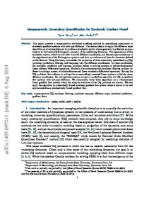
1. Fix some P0 2 IP and let H1 (P ) = kP ? P0 k2 , where k�k stands for the Frobenious norm. Shown in Figure 1 is the evolution of gradient algorithm: plots of H (Pi ) for the iterative values Pi generated by the gradient algorithm.
(6)
The sgn is ?ve to converge to a minima and is +ve to converge to a maxima. Let U be an open neighborhood 3
0.8
1. Diffusion: Stochastic Gradients To avoid local optima this construction is extended to the stochastic gradient and random sampling. If we add a white noise term to the gradient (tangent) vector then it is possible to obtain an equilibrium governed by a steady state invariant measure, say �. This will guarantee visits to all sets in the space with positive �-measure and eventual discovery of the global optimal point. It can be shown that, under certain smoothness constraints on H , the density associated with � ?H (P ) is of the form e Z where Z is the normalizer. The stochastic gradient is generated through the stochastic differential equation:
0.7
0.6
Cost Function
0.5
0.4
0.3
0.2
0.1
0 0
5
10
15 Iteration Index
20
25
30
Figure 1. Gradient steps to find minima of H1 .
dX (t) = ?
2. Let xi ’s be independent realizations of a random variable with the distribution � N (0; aI + bP0 ) and S 1 K xi xy : be the sample covariance matrix S = K i=1 i Maximum-likelihood estimation of P corresponds to the optimization (7)
6.2 6 5.8
Cost Function
5.6 5.4 5.2 5 4.8
4.4
3
4
5 6 Iteration Index
7
8
9
i=1
i;X (t) �dWi (t) ;
Similar to the analysis in Srivastava [12], it can be shown that such a jump-diffusion process samples from the dis?H tribution � with the density e Z . This basic ergodic result relating a jump-diffusion process to the invariant measure � is asymptotic. This implies that, as opposed to the stopping criterion in deterministic gradient case, the result here is achieved in infinite time simulation. Of course, for a computer implementation some stopping criterion has to be chosen depending upon the requirements of the end-user. Algorithms for discrete implementation of jump-diffusion processes are given in Srivastava et. al. [12, 13].
4.6
2
XJ Y
2. Jumps: Model Order Estimation In certain situations the rank m of the subspace may not be known beforehand; the solution can have of any rank from 0 to n. To state the rank explicitly, let IPm be the space of all projection matrices of rank m and let IP = [nm=0 IPm . Let H : IP ! IR+ be a cost function on this disjoint union of sets, each being a connected set. To enable the search process to move across IPm ’s we add a discrete component called a jump process, to the diffusion process. The jumps corresponds to the random transitions across IPm ’s in a pre-defined way. A jump-diffusion process on IP can be constructed using steps similar to the ones described in Srivastava [12] for matrix Lie groups.
The values are chosen to be: a = 2:5, b = 0:5 and K = 20 for the result presented here. Shown in the Figure 2 is the evolution of the gradient program for maximizing the function H2 = trace(PS ) over IP .
4.2 1
i=1
p
i;X (t) H )Yi;X (t) dt+ 2
(8) where � denotes Stratanovich integral and Wi ’s are independent standard Wiener processes. X (t) is called a diffusion process. For an illustration of the discrete implementation of this process through stochastic difference equations, please refer to Srivastava [12].
P
P^ = arg Pmax 2IP trace(PS ) :
XJ (Y
10
Figure 2. Gradient steps to find local maxima of H2 .
4 Jump-Diffusion Flows These gradient algorithms have the drawback that they converge to local optimal points which may not be useful in general. The performance of gradient algorithm will depend upon a good initial condition, in the local neighborhood of the solution, in the sense of Proposition 1.
5 Tracking Rotating Subspaces In certain situations of interest, the observations sample a low-dimensional subspace which is changing in time and 4
at any fixed time there are not enough samples for estimation. We take a statistical approach to tracking subspaces by using a complete Bayesian formulation, including prior dynamic models on subspace rotation. The optimization is performed on the space of trajectories in IP rather than a single point, by extending the algorithm described above. Similar to Fuhrmann et. al. [7], the subspace dynamics is assumed to be modeled by a differential equation of the kind,
[2] William M. Boothby. An Introduction to Differential Manifolds and Riemannian Geometry. Academic Press, Inc., 1986. [3] Roger Brockett. Notes on Stochastic Processes on Manifolds. Systems and Control in the Twenty-First Century: Progress in Systems and Control, Volume 22. Birkhauser, 1997.
dP (t) = A(t) � P (t) ? P (t) � A(t) dt
[4] R. S. Bucy. Geometry and multiple direction estimation. Information Sciences, 57-58:145–58, 1991.
where A(t) is a stochastic process on the space of n � n skew-symmetric matrices. Physically, the elements of A(t) signify the rotational velocities of the rotating subspace represented by the projection matrix P (t). Assuming a probabilistic structure on the process A(t) (perhaps Gaussian with a known covariance), this differential equation can be used to inherit a probability measure on the space of all possible curves P (t), which forms the prior component. This approach is used in Srivastava [12] to impose informative priors on the trajectories of airplane motion. The data likelihood model provides the transition from P to some observation Y to formulate the posterior probability according to the Bayes rule, Prob(P jY ) / Prob(P )Prob(Y jP ). If the posterior probability can be written in a Gibbs’ form Prob(P jY ) = e?HZ(P ) with desired constraints on H , then a jump-diffusion process can be constructed to sample from the posterior and to solve for the conventional estimators such as MAP, MMSE etc.
[5] P. Comon and G.H. Golub. Tracking a few extreme singular values and vectors in signal processing. Proceedings of the IEEE, 78(8), August 1990. [6] L. Conlon. Differentiable Manifolds: A First Course. Birkhauser, 1993. [7] D. R. Fuhrmann, A. Srivastava, and H. Moon. Subspace tracking via rigid body dynamics. Proceedings of Sixth Statistical and Array Signal Processing Workshop, June, 1996. [8] S. Geman and D. Geman. Stochastic relaxation, gibbs distributions, and the bayesian restoration of images. IEEE Transactions on Pattern Analysis and Machine Intelligence, 6(6):721–741, November 1984. [9] U. Grenander and M. I. Miller. Representations of knowledge in complex systems. Journal of the Royal Statistical Society, 56(3), 1994. [10] E. Moulines, P. Duhamel, J. Cardoso, and S. Mayrargue. Subspace methods for the blind identification of multichannel fir filters. IEEE Trans. Signal Processing, 43(2):516–525, February 95.
6 Discussion In this paper we have sketched the construction of: (i) a gradient search algorithm to find the optimal points of a cost function on the space of rank m projection matrices of size n � n (Grassmanian manifold), (ii) extended the deterministic search to jump-diffusion processes to solve for global optimizers when m is unknown. The search processes are intrinsic in that the they stay on the manifold. It should be remarked that these search algorithms may be computationally costly since they include the exponential of n � n skew-symmetric matrices to construct gradient flows. But they are applicable to any cost function H with certain smoothness requirements, not just lower order polynomials.
[11] Steven Thomas Smith. Geometric Optimization Methods for Adaptive Filtering. ph. D. Thesis, Harvard University, Cambridge, Massachusetts, May 1993. [12] A. Srivastava. Inferences on Transformation Groups Generating Patterns on Rigid Motions. D. Sc. Thesis, Washington University, St. Louis, Missouri, July 1996. [13] Anuj Srivastava, Michael Miller, and Ulf Grenander. Ergodic Algorithms on Special Euclidean Groups for ATR. Systems and Control in the Twenty-First Century: Progress in Systems and Control, Volume 22. Birkhauser, 1997.
References [1] K. Abed-Meraim, J.-F. Cardoso, A. Y Gorokhov, P. Loubaton, and E. Moulines. On subspace methods for blind identification of single-input multiple-output fir systems. IEEE Trans. Signal Processing, 45(1):42– 55, January 97.
[14] A.-J. van der Veen, S. Talwar, and A. Paulraj. A subspace approach to blind space-time signal processing for wireless communication systems. IEEE Trans. Signal Processing, 45(1):173–190, January 97.
5