take the malicious nodes as friends and vote for them positively. However .... the evaluation rules to understand how, in real life, trust is established. We have ...
Graph Algebraic Interpretation of Trust Establishment in Autonomic Networks Tao Jiang John S. Baras Institute for Systems Research and Department of Electrical and Computer Engineering University of Maryland, College Park 20742 Email: {tjiang, baras}@isr.umd.edu
Abstract— Trust in networks is the essential foundation for follow-on security mechanisms, such as key management and secure transmission. In this paper, we concentrate on trust establishment in self-organized, distributed and resourceconstraint networks. Such networks pose formidable challenges on trust establishment due to lack of infrastructure and centralized servers. We model our trust establishment strategy as a local voting scheme and discuss its long run behavior. More specifically, we investigate the dynamic evolution of trust within the network, i.e. how trust spreads among nodes, via analyzing its convergence behavior based on algebraic graph and Markov chain theories. As an important security concept, we also study the attack-resistant properties of our trust evaluation scheme in the presence of adversaries.
I. I NTRODUCTION In network security, trust is interpreted as a set of relations among entities participating in network activities. Trust establishment in distributed and resource-constrained networks, such as mobile ad hoc networks (MANETs), sensor networks and ubiquitous computing systems, is considerably more difficult than in traditional hierarchical architectures, such as the Internet and wireless LANs centered on base stations and access points. In traditional networks, sources of trust evidence are centralized control servers, such as trusted third parties (TTPs) and authentication servers (ASs). Those servers are trusted and available all the time. Most prior research efforts in this framework [5], [13], [9] assume an underlying hierarchical structure within which trust relationships between ASs are constrained. In contrast, we are concerned with self-organized networks, which have neither pre-established infrastructures, nor centralized control servers. In these networks, the sources of trust evidence are peers, i.e. the entities that form the network. We summarize the essential and unique properties of distributed trust management in mobile ad hoc networks as opposed to traditional centralized approaches: •
uncertainty and incompleteness: Trust evidence is provided by peers, which can be incomplete and even incorrect. Trust value is continuously ranging between −1 and 1, where −1 stands for complete distrust and 1 for complete trust.
locality: Trust information is exchanged locally. It does not depend on global exchanges since they require high communication costs and do not deal well with fast network changes. • distributed computation: Each agent is its own authority. Trust evaluation is performed individually. To establish trust in such a distributed way has several advantages. Because of locality, it saves network resources (power, bandwidth, computation, etc.), which are limited in a mobile wireless environment. It avoids the single point of failure problem as well. Moreover, the networks we are interested in are dynamic with frequent topology and membership changes, and distributed trust has the desired emergent property as nodes only contact a few and easyto-reach nodes. For scalability and efficiency considerations, trust evaluation is constrained to information provided by directly connected nodes, i.e. it is based on local interactions. Notice that here we mean neighbors in the sense of trust, which have direct trust relations 1 . Our aim is to establish indirect relations between two entities that have not previously interacted; this is achieved by using the direct trust relations that intermediate nodes have with each other. Hence, we assume that trust is transitive, but in a way that takes into account uncertainty also. There have been several works on trust computation based on interactions with one-hop neighbors. In [4], first-hand observations are exchanged between neighboring nodes. Assume Alice receives her neighbors’ opinions about a particular node in the network. Alice merges her neighbors’ opinions if they are close to her opinion on that node. This work provides an innovative model to link nodes’ trustworthiness with the quality of the evidence they provide. In the present paper, we study the inference of trust value rather than generation of direct trust. Our approach is similar with the one used in EigenTrust by Kamvar et al. [7]. In EigenTrust, in order to aggregate local trust values, a node, say i, asks its neighbors of their opinions about •
1 These neighbors are also called logical neighbors as opposed to physical neighbors, which communicate in one hop. Unless otherwise stated, we will use neighbors in the logical sense, and the interpretation neighbors can be inferred from the context.
other peers. Neighbors’ opinions are weighted by the trust i places on them: � cij cjk , (1) tik =
0 0.95 0.9
0.75 0.8
j
where cij is i’s local trust � value for node j and trust values are normalized: ∀i : j cij = 1. To address the adversary collusion problem, they assume there are peers in the network that can be pre-trusted. [10], [16] proposed similar algorithms that evaluate trust by combining opinions from a selected group of users. One possible selection for the selected users is the neighbors. All these algorithms showed promising results against a variety of threat models. However, evaluations in all these works are based on simulations. In this paper, we analyze our local interaction rule using algebraic graph theory and provide a theoretical justification for network management that facilitates trust propagation. In addition to the above works, an extensive amount of research has focused on designing decentralized trustinference protocols, such as [1], [11]. These works categorize trust information broadly into direct trust and recommendations. Trust is evaluated by aggregating trust opinions along and across paths. Such schemes are applicable for networks that are easy to obtain routing and path information, but this is not always true in our setting. This paper is organized as follows. In Sect. II we discuss our framework based on directed graph models. We formally define our trust evaluation rule as a voting scheme. As our main contribution, Sec. III gives theoretical results and provides necessary conditions for establishing a trusted network. Our voting rule is further interpreted as a Markov chain. In Sect. IV, we discuss the impact of topology on our trust establishment procedure and introduce an important graphical parameter, the second largest eigenvalue of a graph, which furthermore guides the network topology design. Section V analyzes our voting rule in the presence of adversaries. The strategies of malicious nodes are modeled and the impact of those malicious nodes on the evaluation rule is investigated. II. P ROBLEM FORMULATION We model the direct trust connections among nodes as a directed graph (digraph) G(V, E), called the trust graph. The nodes of the graph are the users/entities in the network. Suppose that the number of nodes in the network is N , i.e. |V | = N and nodes are labeled with indices {0, 1, . . . , N − 1}. A directed arc from node i to node j, denoted as (i, j), corresponds to the trust relation that entity i, also referred to as trustor, has on entity j, also referred to as trustee. 2 Each arc also comes with a weight called confidence value. The weight function c ij : V ×V → W , where W = [−1, 1], represents the degree of belief i has on j. In a digraph, arcs joining two nodes in the same direction are called parallel 2 Notice that a trust relation from i to j does not necessarily mean that i trusts j. Trust relations include distrust (i.e. negative trust) as well.
3
1
1
1 1 0.9
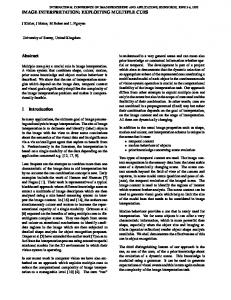
2 Fig. 1.
An example of trust graph
arcs, and a loop is an arc that joins a node to itself. We assume the trust graph is a simple graph without parallel arcs or loops, because a trust relation is considered to be between two distinct entities and it is unique within a given context. The set of i’s neighbors is N i = {j|(i, j) ∈ E} ⊆ {0, . . . , N − 1} \ {i}. Fig. 1 is an example of a trust graph. For a homogenous distributed network, all nodes are equal. There is no reason to specialize any particular node. Therefore, trust evaluation should take all available trust evidence information into account. If node i wants to estimate the trustworthiness of agent j, the natural approach is to aggregate all its neighbors’ opinions on j, which is the trust values the neighbors have on j. It could be interpreted as the following general rule: tij = f (cij , {(cik , tkj )|∀k ∈ Ni and k �= j}) .
(2)
Notice that we do not ask opinions from the target node itself. The function f (·) should satisfy the following properties: • Nodes trust themselves, i.e. t ii = 1; • −1 ≤ f (·) ≤ 1, since our trust value is in the range of [−1, 1]; • Opinions from nodes with high confidence values are more credible, so they should carry larger weights; A. Trust and distrust Distrust is usually ignored in most work on trust management. However, the real world considers distrust to be at least as important as trust. We believe that in the case of adversaries, systems should pay even more attention on distrust information than on trust information, because the damages made by adversaries are usually so severe that systems would not wish to mistake any adversary as a trusted one. In the absence of distrust, it is unclear whether a trust value of 0 means distrust or ‘no opinion’. In our work, we explicitly set trust values between −1 and 1, with distrust as −1 and ‘no opinion’ as 0. So c ik = 0 if i is absolutely uncertain about k or if i has no prior confidence on k. Modeling distrust as negative trust raises several challenges. For instance, how to combine distrusts in a trust chain? Guha etc. in [6] gave three models of propagation
of trust and distrust: trust only, where distrust is completely ignored; one-step distrust, where when i distrusts j, i distrusts all opinions made by j, thus, distrust propagates only one single step; and propagated distrust, where trust and distrust propagate together. From their experiment results, one-step distrust propagation performs the best for most approaches, especially those similar to ours. Therefore, we incorporate distrust using the one-step distrust model. Thus if cij < 0, i will not ask any opinion from j, whereas the negative trust i has on j influences others’ trust evaluation on j. Then the general evaluation rule (2) is modified to incorporate distrust, tij = f (cij , {(cik , tkj )|∀k ∈ Ni , k �= j and cik > 0}) . (3) Notice that tkj can be negative, which represents distrust opinion. B. Weighted voting
distrusted
−1 Fig. 2.
neutral
η−
trusted
η+
The threshold rule on ultimate trust values
format as
� �−1 C +(0) · T (0) (τ − 1), T (0) (τ ) = Z (0)
since only opinions from neighbors with positive confidence are considered, and � zi = c+ ik . k∈Ni
Essentially, in the voting rule, node k, a neighbor of i, votes for target j with the current trust value it has t kj (τ − 1). Node i combines all those votes using weighted average, where weights are equal to i’s direct confidence values on its neighbors. Observe that the computation of t ij is independent of the trust values on any other nodes. The only values that matter are trust values on j and the direct confidence values. So from now on, we only consider trust evaluation on a particular node, say node 0 without loss of generality. Define an (N − 1) × (N − 1) matrix C +(0) = {c+ ij }, i, j = 1, 2, . . . , N − 1, and the trust vector on 0 as T (0) = [t10 , t20 , . . . , t(N −1)0 ]� . Then eqn. (4) is rewritten in matrix
(5)
where Z (0) = diag[z1 , . . . , zN −1 ]. The above equation works for evaluation on other nodes as well. For the sake of simplicity in notation, we omit the index 0 and use the equation in the following form T (τ ) = Z −1 C + · T (τ − 1).
Guided by the above reasoning, we design a simple evaluation rule, which is called the simple voting rule. First we assume direct confidence values are fixed, i.e. for any time τ ≥ 0, cik (τ ) = cik . Generally this assumption is not true, since agents are always willing to adjust their opinions based on new information. However, what we are concerned with within this paper is the convergence of the evaluation rule. By varying the voting values, the convergence time would vary, but eventually trust value converges to the same steady state, given that opinions will be fixed finally. We use tij (τ ) as the trust value of i on j at time (iteration) τ . Then � 1 if i = j �� � tij (τ ) = , + k∈Ni ,k�=j cik tkj (τ − 1) /zi if i �= j (4) where � cij if cij > 0 c+ , ij = 0 otherwise
1
(6)
As τ becomes large, the trust vector will converge to the steady state which decides trust values on the target. We let ti0 = limτ →∞ ti0 (τ ), denote the trust value of i on 0 at the steady state. To distinguish trust values at the steady state and those at any time before convergence, the first are called ultimate trust values, or just trust values for simplicity, and the second are called provisional trust values. Based on the ultimate trust values, entities assess the trustworthiness of the corresponding nodes. The decision varies for different entities and for different contexts. For the convenience of discussion, we apply a threshold rule on the ultimate trust values. The threshold rule is defined through parameters η − and η + as shown in Fig. 2, where trust values range from −1 to 1. Since our voting scheme is purely decentralized, complete trust is not assured beforehand even if all entities are virtuous. The first and indispensable question to answer is how to build up a fully trusted or at least trust connected network in virtuous environments. This is discussed in the next section. III. T RUST SPREADING In this section, we regard the trust establishment process as a dynamical system. In order to evaluate a particular node, trust opinions start from nodes that have direct trust relations with the target. Those opinions spread throughout the network and finally reach all the nodes in the network. We discuss the convergence of the system and investigate the spreading of trust as the system reaches steady state. We start with considering a virtuous network without adversaries, where all nodes behave rationally, i.e., all nodes follow the pre-designed evaluation rule. In this case we have C + = C. To our surprise, the analytic results below show that trust cannot be established under the simple voting rule (4). Then we introduce a new mechanism that helps the establishment of trust.
A. Simple voting Define a matrix M = Z equation (6) is written as
−1
C. Then the state update
T (τ ) = M T (τ − 1) = M τ T (0).
(7)
M can be viewed as a weighted adjacency matrix of the trust graph. It is trivial to verify that M is a stochastic matrix3 . In order to study the properties of M , let’s first introduce some definitions. Definition 1 A permutation of the rows of M with the same permutation applied to the columns is a matrix permutation. We denote by σij the fundamental (i, j)-matrix permutation (interchanging rows i and j and columns i and j). A matrix permutation applied to the adjacency matrix of a graph corresponds to a relabeling of the nodes. We use the notation ◦ for composition of matrix permutations. Definition 2 A matrix M is reducible if there exists a matrix permutation σ = σi1 ,j1 ◦ · · · ◦ σ = σim ,jm such that � M1 0 σ(M ) = , (8) M2 M3 with M1 and M3 square matrices and 0 a zero matrix. Otherwise M is irreducible. A digraph is said to be strongly connected if every node can be reached from every other node following the direction of the edges. It can be shown that a graph, whose (weighted) adjacency matrix is M , is strongly connected if and only if the matrix M is irreducible. This is commonly used as an equivalent definition of irreducibility. If M is reducible, by a certain matrix permutation it can be decomposed as ⎤ ⎡ M11 ⎥ ⎢ .. 0 ⎥ ⎢ . σ � (M ) = ⎢ ⎥ ⎦ ⎣ M1m M2 M3 where M11 , . . . , M1m are irreducible matrices. The convergence behavior of M τ depends on the convergence of those irreducible submatrices, and the component corresponding to M 2 going to 0. Thus results from irreducible matrices can be easily transformed to reducible matrices. However, there are some extreme cases that should be avoided in the voting: • a very fragmented network. We only consider networks that are well connected. • a well connected network with one or a few dangling nodes (nodes that have no outgoing links). These nodes do not trust anyone in the network, thus they cannot contribute to the evaluation process. Only nodes that provide trust information should be included in the trust graph. 3 A matrix is called a stochastic matrix, if the sum of the elements of each row is 1.
From now on, we assume that M is irreducible 4, i.e. the trust graph is strongly connected. Since M is a stochastic matrix, the largest eigenvalue of M is 1. Let row vector π be the left eigenvector ( a row vector) corresponding to eigenvalue 1 with |π| = 1, then πM =π 5 . We could prove by ergodicity [12] that, ⎤ ⎡ π ⎢ π ⎥ ⎥ ⎢ lim M τ = ⎢ . ⎥ . τ →∞ ⎣ .. ⎦ π Thus ∀i, 1 ≤ i ≤ N − 1, ti0 = lim ti0 (τ ) = π × T (0) = τ →∞
N −1 �
πj tj0 (0).
j=1
Since ti0 is independent of i, every node reaches the same trust value at the steady state. We can see that trust values purely depend on the initial trust vector T (0). If a node is trusted by a large portion of nodes in the network at the beginning, its trust values are high at steady state. However, in distributed networks, initially only a small number of nodes have direct trust relations with the target, i.e. T (0) is sparse with a few non-zero entries. In addition, entries of π are usually small when N is large. For instance, consider a k-regular graph in which all arcs are with confidence value 1. Then the left eigenvector π = [ N1−1 , . . . , N 1−1 ]� . Since the trust graph is sparse, k N , we have k
1. ti0 = N −1 The result indicates that even in a network with all neighbors’ confidence values equal to 1, the trust values at steady state are very small, i.e. close to 0. Thus under the simple voting rule, it is almost impossible to establish trust even when all voting values are 1. This actually emphasizes the difficulties of designing algorithms in selforganized distributed networks. In order to overcome the above problem, in the next section we introduce the notion of headers, which are entities always trusted by some nodes with trust value 1. B. Voting with headers As we just mentioned, headers are pre-trusted entities. For instance, they can be leaders of clusters, or entities holding a certificate signed by authorities. An entity can be considered as a header only if it has been proven to be reliable and attack-resistant. Notice that the notion of headers does not violate our assumptions for distributed networks. Headers are different with centralized authorities, since nodes can choose to believe in different headers and 4 Convergence properties of M are related to the period of M as well. We assume M is aperiodic without further discussion. A nonnegative matrix is primitive if it is irreducible and aperiodic. 5 In the literature, π is usually called the dominant or principle eigenvector.
a header is not required to be trusted by the whole network. Furthermore, we allow uncertainty in headers’ opinions. Define the number of headers i trusts as y i and the algebraic average of votes provided by those y i headers for node 0 as bi . Let the matrix Y = diag[y 1 , . . . , yN −1 ] and the vector B = [b1 , . . . , bN −1 ]� . Then the updating rule in (6) changes to (9) T (τ ) = (Z + Y )−1 (CT (τ − 1) + Y B) . We first discuss convergence of the above voting scheme. Theorem 1: If the trust graph is strongly connected (C is irreducible), the trust vector converges to a unique trust vector with T = (Z + Y − C)−1 Y B (10)
�
Proof: We write (9) in the following form � � T (τ ) (Z + Y )−1 C (Z + Y )−1 Y T (τ − 1) (11) = 0 I B B
Let M� =
�
(Z + Y ) 0
then (M � )τ = where X(τ ) =
−1
−1
C (Z + Y ) I
�� �τ (Z + Y )−1 C 0
Y
,
X(τ ) , I
�� � �τ −1 (Z + Y )−1 C + · · · + I (Z + Y )−1 Y.
Since the matrix (Z +Y )−1 C is a substochastic matrix with determinant less than 1, we have � �τ I + (Z + Y )−1 C + · · · + (Z + Y )−1 C + · · · =(Z + Y − C)−1 (Z + Y ). Thus, we can get the limit for X(τ ), X = lim X(τ ) = (Z + Y − C)−1 Y τ →∞ � �τ In addtion, we know (Z + Y )−1 C goes to 0. Then, � � � T (τ ) 0 X T (0) = , lim B 0 I B τ →∞ and T = lim T (τ ) = XB = (Z + Y − C)−1 Y B. τ →∞
We can see that the trustworthiness of node 0 is a function of the number of headers and their votes for it. In order to increase its trust values to be above the threshold η + , node 0 needs to gain higher trust from the headers. More interestingly, the voting scheme can be interpreted as a Markov chain on a weighted directed graph. Each node is a state in the Markov chain with transition matrix M � . Suppose we are considering the trust value t i0 . The Markov chain starts from state i, and choose the next (τ ) state according to the transition matrix. Define p ij as the
1
0 0.75 0.75
h 1
0.8
3
1
1
1 1 0.9
2 Fig. 3. Markov chain for trust evaluation of node 0. Dotted lines denote direct confidence values and node h is the header whom node 3 trusts.
probability that the Markov chain is in node j at time τ . Then the provisional trust value represents the expected trust value at current time, which is � (τ ) ti0 (τ ) = pij tj0 (0). j∈V
From the transition matrix, headers are actually absorbing states in the Markov chain, which have no outgoing link. Then the previous trust graph (Fig. 1) can be modified to represent the evaluation of node 0 as a Markov chain, as shown in Fig. 3. The Markov chain will eventually stop in one of the absorbing states. Assume the probability of stopping in header h starting from i is q ih and the trust value of h on node 0 is v h0 . Then there is an alternative explanation for the ultimate trust value � ti0 = qih vh0 . (12) h∈H
We can use the first-step analysis [2] to compute the absorption probabilities q ih . The results are equivalent to the ones in Theorem 1. The Markov chain interpretation also gives more insights regarding the feasibility of our voting scheme. Intuitively, the Markov chain can be viewed as a random walk on the digraph. Assume that a mobile agent is moving on the digraph according to the transition matrix. It tends to choose the neighbor with high transition probability as the next hop. Transition probabilities depend on the confidence values. Therefore the mobile agent has a tendency to visit nodes that are highly connected and with high confidence values. So the expected trust values take more weights on highly connected and highly trusted nodes, which usually provide relatively accurate information. IV. C ONVERGENCE RATE AND NETWORK TOPOLOGY Having found a simple and localized trust establishment method, the next concern is the dynamics of the trust establishment procedure. Especially, in mobile networks, how fast the procedure reacts to network changes is particularly important. So the time it takes to reach the steady state should be taken into consideration; in other words a good scheme should have fast convergence rate.
1
2
second largest eigenvalue (λ )
0.99
0.98
0.97
0.96
0.95
0
2
Fig. 4.
4
6
8 10 12 number of edges added
14
16
18
20
The second largest eigenvalue λ2
5000
4500
4000
3500 convergence time (round)
First, we introduce an important theorem for non-negative matrices, the Perron-Frobenius Theorem [12], which states that for a nonnegative primitive matrix A, there exists a real eigenvalue λ 1 with algebraic as well as geometric multiplicity 1 such that λ1 > 0, and λ1 > |λj | for any other eigenvalue λj . By matrix decomposition, we also have that An = λn1 v1 uT1 + O(nm2 −1 |λ2 |n ) ,where u1 and v1 are the left and right eigenvectors respectively associated with λ 1 , λ2 is the second largest eigenvalue and m 2 is the algebraic multiplicity of λ2 . For a stochastic matrix, λ 1 = 1 and |λ2 | < 1. We also know v1 = 1 and u1 = π. Thus the convergence rate of A n is of order nm2 −1 |λ2 |n . Since our voting rule (9) can be written as eqn. (11), the convergence rate depends on M � . Therefore, the idea is to reduce λ2 of M � . Then the question becomes: what kind of networks or which network topology has smaller λ 2 ? In 1998, Watts and Storgatz [15] proposed their famous smallworld model. Since then, research on network topology has gained voluminous attention. The small world models have two prominent properties: high clustering coefficient and small average graph distance between any pairs. The small average distance essentially indicates that nodes can communicate with other nodes in a few hops given a very large network. In this paper, we consider one of many small-world models, the so-called ϕ-model [14], which is modeled by adding a small number of new edges into a regular lattice. The network starts from a two-dimensional lattice with periodic boundary, and the neighbors are those one hop away. Then new edges are added by randomly choosing two unlinked nodes. In our simulations, a network is considered with 400 nodes on the lattice. For the original lattice, each node has 4 neighbors, and the total number of edges is 800. Each simulation includes several rounds. At each round, 2 new edges are added randomly into the network. The second largest eigenvalue and the convergence time are computed for each round. Fig. 4 shows the second largest eigenvalue λ2 as a function of the number of new edges added. It shows that with more edges added, the second largest eigenvalue of the graph decreases. So, generally speaking, most smallworld networks have smaller second largest eigenvalue than the original lattice. Fig. 5 illustrates the substantial changes of the convergence time as new edges are added. Notice that when 8 new edges are added, which is just 1% of the total edges, the convergence time drops from 5000 rounds to 500 rounds. Thus trust is established much faster in a network with small-world property than a regular lattice. This observation gives rise to a new direction for the construction of the trust graph. Because of resources constraints, each entity can have trust relations with only a few entities, thus the trust graph is sparse. A sparse graph usually has very slow convergence rate, which leads to slow updates for network mobility. From the above observation, the performance of the voting scheme can be improved by introducing shortcuts, i.e. establishing trust relations directly between pairs of entities instead of using several
3000
2500
2000
1500
1000
500
0
0
2
4
6
Fig. 5.
8 10 12 number of edges added
14
16
18
20
Convergence time
hops between them in the trust reference graph. As we have seen, just 1% of new shortcuts can greatly reduce the convergence time. Obviously, to set up shortcuts requires more communication and computation cost. The tradeoff between the number of shortcuts (and the associated cost) and network performance will be an interesting problem to study. V. S ECURITY ISSUES The objective of trust establishment is to exclude misbehaving entities and reduce risks in future communications. In this section, we study the effects of malicious entities on our voting scheme. Since we are focusing on the voting scheme, the security assumptions are limited to the votes entities provide and the evaluation policies they use. We assume the malicious nodes are powerful, thereby strengthening our negative results. Malicious nodes can accurately tell who are their friends, malicious nodes as well, and who are good ones, their votes and evaluation policies are arbitrary. Besides, we consider the case that non-header nodes may mistakenly take the malicious nodes as friends and vote for them positively. However, headers, as the definition implies, are more reliable. They are able to detect misbehaviors and vote for malicious nodes with negative value (possibly not −1). Also, the evaluation policy employed by all virtuous nodes is the voting scheme we previously defined. We start from
⎛
1 1
0
m
−1
0.75 0.75
h
⎞ 0.9 1 0 1 ⎠, 0 0
⎛
⎞ −1 B = ⎝ 0 ⎠. 0.75
1
Then we have
0.8
0.2
0 C=⎝ 0 1
3
1
1
1 1 0.9
2
T = [0.45, 0.60, 0.60]�, compared to the original T = [0.75, 0.75, 0.75] � without the malicious node. C. Collusion of adversaries
Fig. 6. Markov chain for evaluation of node 0 with presence of malicious node m. Dotted lines denote direct confidence values.
a single adversary in the network, and then discuss cases with collusion of adversaries. A. Detecting a single adversary By eqn. (12), for any header h, if the direct trust it has on the adversary m satisfies v hm < η − , all the ultimate trust values on m are below η − , i.e., m is detected. Therefore, even though some non-header nodes mistakenly provide positive votes about the adversary at the beginning, these wrong opinions fade away as the system evolves. Since headers connected to high confidence nodes have higher weights, the conditions on correct detection can be relaxed. Wrong opinions from lowly trusted headers can be compensated by accurate opinions of highly trusted headers. Apparently, headers play very crucial roles in the voting scheme. Entities need to select headers with much caution. B. Impact of malicious votes In distributed trust establishment, the adversary also contributes to the evaluation for other nodes. The trivial case is when none of the good nodes has positive opinion on the adversary. Because one-step distrust is used, none will consider opinions of the adversary. There is nothing the adversary can do for the trust evaluation. This is actually one advantage of the one-step distrust model. However, in a distributed scenario, we cannot exclude the case that the adversary cheats to gain trust from some good nodes; then the votes provided by the adversary are also propagated into the network. The goal of adversaries is to reduce the trust value of the target as much as possible by choosing their strategies of voting and evaluation. We assume that the adversary employs the worst-case strategy which minimizes the trust value: it always votes −1 on good nodes and never changes its votes. In view of the Markov chain, the adversary using the worst-case strategy is also modeled as a header with v m0 = −1. Fig. 6 shows an example, where node 1 mistakenly trusts the malicious node m with confidence value 0.2. We could compute the trust value using eqn. (10) with Z = diag[1.9, 1, 1],
Y = diag[0.2, 0, 1],
Now we consider more than one, say M , adversaries are present in the network. According to our assumptions, these adversaries know each other and are able to collude in order to achieve the maximum destruction to the voting scheme. Similarly as in the above argument, the worst-case strategy of these M adversaries is to always vote −1 for good nodes and reversely 1 for other adversaries, and they never change their votes. So adversaries are also modeled as absorbing states. Suppose the system is evaluating a good node, say 0. Assume that there are H headers and their votes on node 0 are denoted by v h0 , for an arbitrary header h. For simplicity, we assume the trust graph is ideally regular in the sense that the absorption probabilities of headers and adversaries are the same, denoted as q. Apparently q(H + M ) = 1. We have that the trust value is � qvh0 − qM, t0 = h
which is the same for all the evaluating nodes. Then we could estimate the security impact as a function of the number of adversaries. According to the threshold rule, if t < η + , then we have � node 0 is not trusted + q( h v� h0 − M ) < η . So if the number of adversaries M > ( h vh0 − η + H)/(1 + η + ) = M ∗ , the scheme fails in assessing the trustworthiness of node 0. Therefore, M ∗ is the attack-resistant threshold for the voting scheme. In a more realistic scenario, entities with low confidence values are easy to be cheated by adversaries. Adversaries that link to low trusted entities have lower absorption probabilities, then the attack-resistant threshold is actually greater than M ∗ , i.e. the scheme resists more adversaries. The arguments of detecting adversaries are similar with the evaluation, except that the number of adversaries as absorbing states is M − 1 instead of M , since the M th adversary is now the evaluating target. VI. D ISCUSSION In this paper, we formally defined a trust establishment strategy based only on local interactions. We showed the difficulties of establishing trust in a distributed manner and introduced a new notion of headers which help in distributed trust establishment. We studied the convergence behavior of the scheme we proposed using algebraic graph theory and also interpreted it as a Markov chain on a digraph. Furthermore, we discussed the topology effects on
trust spreading, which enlightens a new way for network management. In the last part, since trust management is an important component of network security, issues about trust establishment in the presence of adversaries were investigated. Our approach shares many similarities with work on algorithms for search engines, such as PageRank [3] and HITS [8]. The rank of pages on the network can be viewed as their trust values. Due to the tremendous success of Google, the underlying algorithms have been carefully studied. It would be interesting to relate those search engine algorithms with our trust establishment scheme. Though our weighted voting rule is primitive, it is the starting point of our exploration on how trust is built up in a purely decentralized network. Furthermore, we would like to study more delicate evaluation rules, such as nonlinear rules, adaptive rules and rules for distrust information dissemination. More significantly, we will abstract trust data from real communication experiments and formally model the evaluation rules to understand how, in real life, trust is established. We have discussed the impact of network topology on convergence rate. There are also several interesting problems regarding the trust graph management. For instance, we would like to study the sensitivity of the evaluation rule as the topology changes. The cost tradeoff between modification of the trust graph topology and the performance of trust evaluation is also of great interest. R EFERENCES [1] T. Beth, M. Borcherding, and B. Klein, “Valuation of trust in open networks,” in Proceedings of 3rd European Symposium on Research in Computer Security – ESORICS’94, 1994, pp. 3–18. [2] P. Br´emaud, Markov chains: Gibbs fields, Monte Carlo simulation, and queues, ser. Texts in Applied Mathematics; 31. Springer-Verlag New York, Inc., 1999. [3] S. Brin, L. Page, R. Motwami, and T. Winograd, “The PageRank citation ranking: bringing order to the web,” Computer Science Department, Stanford University, Tech. Rep. 1999-0120, 1999. [4] S. Buchegger and J.-Y. L. Boudec, “The effect of rumor spreading in reputation systems for mobile ad-hoc networks,” in Proceedings of Modeling and Optimization in Mobile, Ad Hoc and Wireless Networks (WiOpt), Sophia-Antipolis, France, 2003. [5] V. D. Gligor, S.-W. Luan, and J. Pato, “On inter-realm authentication in large distributed systems,” in Proceedings of the IEEE Conference on Security and Privacy, 1992, pp. 2–17. [6] R. Guha, R. Kumar, P. Raghavan, and A. Tomkins, “Propagation of trust and distrust,” in Proceedings of International World Wide Web Conference, New York, NY, May 2004. [7] S. D. Kamvar, M. T. Schlosser, and H. Garcia-Molina, “The EigenTrust algorithm for reputation management in P2P networks,” in Proceedings of the 12th Initernational World Wid Web Conference, Budapest, Hungary, 2003, pp. 640–651. [8] J. Kleinberg, “Authoritative sources in a hyperlinked environment,” Journal of the ACM, vol. 46, no. 5, pp. 604–632, 1999. [9] B. Lampson, M. Abadi, M. Burrows, and E. Wobber, “Authentication in distributed systems: Theory and practice,” in Proceedings of the 13th ACM Symposium on Operating Systems Principles, Oct 1991. [10] S. Marti and H. Garcia-Molina, “Limited reputation sharing in P2P systems,” in Proceedings of the 5th ACM conference on Electronic commerce. New York, NY, USA: ACM Press, 2004, pp. 91–101. [11] U. Maurer, “Modelling a public-key infrastructure,” in Proceedings of 1996 European Symposium on Research in Computer Security – ESORICS’96, 1996, pp. 325–350.
[12] E. Seneta, Non-negative matrices and Markov chains, 2nd ed., ser. Springer series in Statistics. Springer-Verlag New York Inc., 1981. [13] J. Steiner, C. Neuman, and J. I. Schiller, “Kerberos: An authentication service for open network systems,” in USENIX Workshop Proceedings, UNIX Security Workshop, 1988. [14] D. J. Watts, Small Worlds: the dynamics of networks between order and randomness. Princeton University Press, 2004. [15] D. J. Watts and S. H. Strogatz, “Collective dynamics of “small-world” networks,” Nature, vol. 393, pp. 440–442, 1998. [16] L. Xiong and L. Liu, “PeerTrust: Supporting reputation-based trust in peer-to-peer communities,” IEEE Transactions on Knowledge and Data Engineering, Special Issue on Peer-to-Peer Based Data Management, 2004.