Graph-Based Multi-Surface Segmentation of OCT ... - Semantic Scholar

TRANSACTIONS ON MEDICAL IMAGING, VOL. XXX, NO. XXX, MONTH YEAR

1

Graph-Based Multi-Surface Segmentation of OCT Data Using Trained Hard and Soft Constraints Pascal A. Dufour*, Lala Ceklic, Hannan Abdillahi, Simon Schr¨oder, Sandro De Dzanet, Ute Wolf-Schnurrbusch, Jens Kowal

Abstract—Optical Coherence Tomography is a well established image modality in ophthalmology and used daily in the clinic. Automatic evaluation of such datasets requires an accurate segmentation of the retinal cell layers. However, due to the naturally low signal to noise ratio and the resulting bad image quality, this task remains challenging. We propose an automatic graphbased multi-surface segmentation algorithm that internally uses soft constraints to add prior information from a learned model. This improves the accuracy of the segmentation and increase the robustness to noise. Furthermore, we show that the graph size can be greatly reduced by applying a smart segmentation scheme. This allows the segmentation to be computed in seconds instead of minutes, without deteriorating the segmentation accuracy, making it ideal for a clinical setup. An extensive evaluation on 20 OCT datasets of healthy eyes was performed and showed a mean unsigned segmentation error of 3.05 ± 0.54µm over all datasets when compared to the average observer, which is lower than the inter-observer variability. Similar performance was measured for the task of drusen segmentation, demonstrating the usefulness of using soft constraints as a tool to deal with pathologies. Index Terms—Segmentation, optical coherence tomography, optimal net surface problems, retina, ophthalmology.

O

I. I NTRODUCTION

PTICAL Coherence Tomography (OCT) is an image modality that allows the in-vivo imaging of biological tissue. In ophthalmology it is used for diagnostic purposes, as it allows the non-invasive, high resolution imaging of the intraretinal cell layers. With the advances in image quality and acquisition speed, such as the Spectral Domain OCT methods, the amount of data that has to be inspected by the clinician is ever increasing. Automatic segmentation of the retinal layers aims to reduce the time required to screen OCT datasets, evaluate them and state a diagnosis. Quantitative thickness measurements and topographic thickness maps provide valuable information of a patient’s retinal cell layers and are widely used for both diagnostic and scientific purposes [1]. However, Asterisk indicates corresponding author *P. A. Dufour, S. De Zanet and Jens Kowal are with the ARTORG Center for Biomedical Engineering Research at the University of Bern, 3010 Bern, Switzerland and the University Hospital Bern, Department of Ophthalmology, 3010 Bern, Switzerland (emails: [email protected], [email protected], [email protected]). L. Ceklic, H. Abdillahi, S. Schr¨oder and U. Wolf-Schnurrbusch are with the University Hospital Bern, Department of Ophthalmology, 3010 Bern, Switzerland and the Bern Photographic Reading Center, 3010 Bern, Switzerland (emails: [email protected], [email protected], [email protected], [email protected]). c 2010 IEEE. Personal use of this material is permitted. However, permission to use this material for any other purposes must be obtained from the IEEE by sending a request to [email protected]. The original paper can be accessed at IEEE Xplore. Digital Object Identifier 10.1109/TMI.2012.2225152

these measurements require an accurate segmentation. Due to the difficulty of the problem, current commercially available tools only provide very limited segmentation capabilities, restricting the segmentation to two or three layers, and segmentation of images with bad quality often fails. An automatic segmentation method should be fast, accurate and robust to image degradation and low signal-to-noise ratio. The possibility of segmenting pathologies is also highly desired. Many approaches for multi-surface intraretinal layer segmentation have been published, but either the computation time is in the order of minutes (or even hours) instead of seconds, or the accuracy and robustness suffers, making them infeasible for a clinical setting. We quickly highlight the current state of the art in intraretinal layer segmentation. Yazdanpanah et al. use an active contour approach for the segmentation of rodent retinas [2]. Their method makes use of region-based, shape prior and regularization energy terms. This helps in the presence of speckle noise, but requires a good initialization. Unfortunately, their method was never tested on OCT datasets of human retinas, and it is not clear how well this method can handle the morphological abnormalities present in pathologies. A two-step kernel-based optimization was proposed by Mishra et al. [3]. An initial approximate segmentation is refined using a force balance equation based on dynamic programming. However, the experiments were only performed on rodents. A method by Zhang et al. is based on locally weighted gradient extrema [4]. A statistical error estimation techniques is then applied to eliminate outliers. However, the method was never evaluated on pathological datasets. Instead of using gradients, Fabritius et al. use intensity variations in OCT signals for segmentation [5]. While the method is relatively fast, only two boundaries are detected. Yang et al. published an approach that simultaneously uses global gradient information and local canny edge detection [6]. Dynamic programming is then applied to smooth the detected edges. Vermeer et al. employ machine learning to classify each pixel in an OCT volume as belonging to a specific cell layer [7]. Level set methods are then used to regularize the classified pixels to eliminate outliers. In theory, this method could work well with pathologies if the training dataset contains enough examples of pathologies, but this was not yet evaluated. A graph-based algorithm to segment intraretinal layer boundaries using dynamic programming was introduced by Chiu et al. [8]. This method was then also applied to the segmentation of datasets from patients with agerelated macular degeneration (AMD) [9], showing accurate results for images of low quality. Their algorithm processes B-scans individually, which is valuable if no volumetric data

Copyright 2012 IEEE. The original paper can be accessed at IEEE Xplore. Digital Object Identifier 10.1109/TMI.2012.2225152

TRANSACTIONS ON MEDICAL IMAGING, VOL. XXX, NO. XXX, MONTH YEAR

is available. On the other hand, information from neighboring B-scans is not used when segmenting a volume. However, an extension to their algorithm using an iterative dynamic programming approach could make full use of the volumetric information. Haeker et al. uses a different graph-based method that allows the simultaneous searching of multiple interacting surfaces in time-domain OCT [10]. Garvin et al. subsequently extended the method to spectral domain OCT volumes and included varying feasibility constraints, which greatly improved the segmentation [11]. A graph-based approach such as this finds the globally optimal segmentation with respect to the cost function. However, the high amount of speckle noise is difficult for a graph-based approach because there is no regularization as with active contour approaches or dynamic programming. One way of overcoming this limitation was proposed by Antony et al. by including texture information into the segmentation process [12]. Features were computed using Gabor filters and a k-NN classifier was applied to compute probability maps for each cell layer. Including this information in the cost function for the segmentation yielded improved results compared to a purely gradient-based cost function. Another method is to incorporate regularization terms directly into the graph. This was demonstrated by Song et al. for the segmentation of bladder and prostate [13] and was later also used on OCT volumes [14]. This regularization was made possible by adding soft constraints. Soft constraints do not limit the feasibility of a segmentation, but rather impose an additional cost if the segmentation deviates from an expected model. Whenever any such soft constraint is violated, the solution is still valid, but has a higher cost than when it would not be violated. Thus, they help driving the solution towards a specified model, which can be learned from manual segmentation and helps incorporating prior information into the segmentation. We build on their work and extend the framework by Song et al. [14]. While their work only describes how soft constraints can be applied to regularize the shape of the segmented surfaces, we extend the method to allow for soft constraints that can also be applied to the regularization of the distances between two simultaneously segmented surfaces. Furthermore, we describe how the soft shape constraint can be added to a neighborhood instead of only to a node. This decreases the introduced error from discretizing the learned model and thus leads to a more accurate soft constraint, which means the dataset can be segmented without flattening it beforehand. In the following sections, each used soft constraint is explained at a high, abstract level and compared to its corresponding hard constraint. We then show how to incorporate these constraints into the graph. Furthermore, we also describe how the graph size can be reduced using the same prior model, resulting in an algorithm that runs in seconds instead to minutes and requires less than 1GB of memory, making it feasible for a clinical setup. Finally, an extensive evaluation is performed to demonstrate the superior quality of the segmentation for fovea centered OCT scans of normal subjects. Because the soft constraints

2

make the segmentation of pathologies easier, we test the performance of the proposed algorithm on the segmentation of drusen in OCT datasets of patients with age-related macular degeneration. We also test how well the algorithm performs in the presence of artificially added speckle noise. II. M ETHODS The segmentation problem is stated as an energy minimization problem that is solved with the optimal net surface problem [15]. Let S be a set of surfaces S1 to Sn , then the energy of the segmentation is given by E(S) =

n X

(Eboundary (Si ) + Esmooth (Si ))

i=1

+

n X1

n X

Einter (Si , Sj )

(1)

i=1 j=i+1

The external boundary energy Eboundary (Si ) is computed purely from the image data. This can be seen as a force that pushes the surface toward the best fit in the image. The surface smoothness energy Esmooth (Si ) guarantees the connectivity of a surface in 3D and regularizes the surface. Intuitively, this defines how rigid a surface is and how easy it can be deformed. The interaction energy Einter (Si , Sj ) constrains the distance of surface Si to surface Sj . This acts like a force between two surfaces, pushing or pulling them towards a specified distance of each other. At the core of the algorithm is the prior information model that is used for both the hard and soft constraints. We first illustrate how it can be built from training datasets. The design of each energy term in (1) is then described in the following sections. A. Prior Information Model The prior information model is a statistic on the distance between surfaces in relation to the fovea position. It is composed of multiple mean models, keeping track of the mean distance between two surfaces, and corresponding variance models, describing the variance of the distance between those surfaces. The model was built from 28 training datasets consisting of segmentations of fovea-centered OCT slice stacks. Each OCT slice stack comes from a different patient and is first automatically segmented using the method described by [11]. The segmentations were then manually corrected with a custom built application. To make the model more accurate, the location of the fovea was used as an anchor. We now describe how this model can be built, given n training datasets. First, the location of the fovea is found by searching for the lowest point on the segmented internal limiting membrane (ILM). This was needed because most of the standard OCT images from the clinic are not perfectly centered at the fovea. Furthermore, because our datasets had a high lateral resolution within B-scans, but a low resolution between subsequent B-scans, sub-pixel accuracy was required. To achieve this, we implemented a simple local optimization

Copyright 2012 IEEE. The original paper can be accessed at IEEE Xplore. Digital Object Identifier 10.1109/TMI.2012.2225152

TRANSACTIONS ON MEDICAL IMAGING, VOL. XXX, NO. XXX, MONTH YEAR

3

120!m

80!m

40!m

0!m

(a)

(b)

(c)

(d)

(e)

(f) 30!m

20!m

10!m

0!m

(g)

(h)

(i)

(j)

(k)

(l)

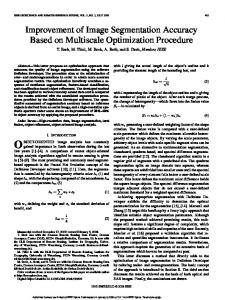
Fig. 1. Prior information model, consisting of mean and variance models used to incorporate prior local information into the graph. As a reference, the axial pixel resolution of the used OCT volumes is 3.9µm. (a) Mean nerve fiber layer thickness, (b) combined mean ganglion cell and inner plexiform layer thickness, (c) combined mean inner nuclear and outer plexiform layer thickness, (d) mean outer nuclear layer thickness, (e) mean retinal pigment epithelium thickness and (f) used color function for the mean thickness maps. The second row shows the corresponding variance models as standard deviations to the mean thickness maps.

procedure that finds the circular area with a predefined radius on the segmented surface of the internal limiting membrane (ILM) with the lowest average height. All n training datasets are then translated in 3D so that the fovea of each dataset is at the coordinate origin. The mean model mi,j µ : (x, y) ! R, describing the mean distance between the surfaces Si and Sj of the n datasets, can then be computed by sampling the n training segmentations at predefined sampling locations (x, y). n

mi,j µ (x, y) =

1X k Si (x, y) n

Sjk (x, y)

(2)

k=1

The variance model mi,j : (x, y) ! R, describing the variance of the mean distance between surface Si and Sj , is computed in the same fashion. Note that we only built a model for the right eye. However, the laterality can easily be switched by mirroring the model around the sagittal plane. Fig.1 shows the mean and variance models for a few selected layers. B. Boundary Energy The approach from Li et al. [15] is used to construct the graph. For completeness, we quickly review the basic steps required for multi-surface segmentation. For a more detailed description, see [11], [15], [16]. Using the multicolumn model notation from Li et al., the image I(x, y, z) can be viewed as a set of columns defined by their x- and y-coordinates. Every voxel in the volumetric image becomes a node V (x, y, z) in the graph. Every column is intersected by the surface Si exactly once. Therefore, Si can be defined by a function fi : (x, y) ! z that assigns a height to each column.

Given a surface Si , the boundary energy Eboundary (Si ) describes its fit to the image data. Let ci : (x, y, z) ! R be the cost function defining the inverse likelihood of surface Si belonging to the node V (x, y, z). The weight assigned to node V (x, y, z) is then defined as ⇢ ci (x, y, z) if z = 0 wi (x, y, z) = (3) ci (x, y, z) c(x, y, z 1) otherwise We first apply anisotropic filtering [17] on the original image and then compute ci from the gradient in the filtered image. The problem of finding the globally optimal segmentation can be solved by finding the minimum closure in a derived arcweighted graph. A directed graph is called closed if it has no outgoing edge. The minimum closure problem is then to find the closed set that has the minimal combined node weights. To make sure that the solution of the minimum closure problem is not simply the empty set (with zero cost), a negative constant is added to the cost ci (x, y, 0) for Vi (x, y, 0), the lowest node in column (x, y), called the base node of that column. Furthermore, all base nodes are connected to their neighboring base nodes with undirected edges. Now, the solution of the minimum closed set that includes all base nodes would be the sum of the costs of those nodes, which is negative. This guarantees that the surface cuts each column above its base node. To ensure that the surface intersects each column exactly once, directed intra-column edges are created. They connect each node V (x, y, z) to V (x, y, z 1), the node below in the same column. Intuitively, since the minimum closure cannot have any outgoing edges, if a specific node in a column belongs to the minimum closure, all nodes below in the same column must also belong to the minimum closure. An example with two neighboring columns is Fig.2, showing these intracolumn edges and the edges connecting the base nodes in gray.

Copyright 2012 IEEE. The original paper can be accessed at IEEE Xplore. Digital Object Identifier 10.1109/TMI.2012.2225152

TRANSACTIONS ON MEDICAL IMAGING, VOL. XXX, NO. XXX, MONTH YEAR

col(x, y) col(x + 1, y)

max (x, y) x

=3 min x (x, y)

=1

Fig. 2. Example graph including a hard smoothness constraint with two columns. All edges have infinite costs. The surface height at column (x + 1, y) may not be more than 1 node lower than the surface height in column (x, y) (blue inter-column edges going from column (x, y) to column (x + 1, y)). At column (x + 1, y), the surface height must not be more than 3 nodes higher than the surface height in column (x, y) (green inter-column edges, going from column (x + 1, y) to column (x, y)). A surface must further cut each column exactly once, guaranteed by the grey intra-column edges. A violation of any of the above constraints would result in at least one cut edge with infinite cost, thus rendering the solution infeasible.

C. Smoothness Energy The energy term for the smoothness of a surface limits its height difference between neighboring columns. The term is split up in hard and soft energy terms: Esmooth (Si ) = EsmoothHard (Si ) + EsmoothSoft (Si )

(4)

In Garvin et al. [11], only the hard smoothness constraint was used. This constraint limits the height differences between neighboring columns to a specified value. A 4-connected neighborhood is used in this work: every (x, y)-column is considered adjacent to the (x 1, y)-, (x + 1, y)-, (x, y 1)and (x, y + 1)-columns. For every node V (x, y, z), the minimum height difference to the neighboring columns is given by a value min x (x, y) specifying the maximum allowed height decrease in x-direction, and max (x, y), the maximum allowed height increase in xx direction at position (x, y). In y-direction, min y (x, y) and max (x, y) define the same constraints. y To incorporate this constraint into the graph, directed intercolumn edges are created between adjacent columns. Given two columns (x, y) and (x0 , y) that are adjacent in x-direction, min edges are added from V (x, y, z) to V (x0 , y, z x (x, y)) 0 max and to V (x , y, z + x (x, y)). This is done for every node in the column (x, y). In y-direction, the edges are connected in the same fashion with the values from min y (x, y) and max (x, y). Fig.2 illustrates this concept. y Note that these values depend on the (x, y)-positions in the graph. By varying the terms min and max over the position, prior information can be incorporated. This was presented by Garvin et al. in [11]. The above described minimum closure problem can be solved with a minimum s-t cut, as described in [15], [16]. Every edge (intra- and inter-column edges) in the described minimum closure problem becomes an edge with infinite cost in the graph for the minimum s-t cut. Note that edges with infinite costs cannot be cut in a minimum s-t cut, therefore the cut solves the closure problem. Additionally, there are two new nodes, the source and sink nodes. The source is connected to every node from the minimum closure problem with a directed edge of cost w, and every node from the minimum closure problem is connected to the sink with a directed edge of cost w. Here, w refers to the previously defined weight for a node in the minimum closure problem. While the infinite edges

4

only guarantee that the solution of the minimum s-t cut is a closure, the new edges from the source to the nodes and from the nodes to the sink guarantee the solution is indeed the minimum closure. For a more detailed explanation, we refer the reader to the papers by Wu et al. [16] and Li et al. [15]. The described smoothness constraint is considered a hard constraint because it limits the feasible surface, due to the fact that the weights of the edges are infinite. If instead a finite value is used, it would only impose a penalty when the constraint is violated. This concept is applied here to incorporate soft smoothness constraints. The soft constraint is intended to punish the deviation from a given prior model, but not prohibit it. Song et al. first described the soft smoothness constraints using directed edges and show how an arbitrary convex function can be incorporated into the graph [14]. In contrast, we use only undirected edges, which leads to a simpler formulation, but essentially allows to add the same constraint. We start by adding a linear constraint on the deviation of the first derivative from the prior shape: ⇣ P EsmoothSoft (Si ) = x2X wix · fi (x,y) mi x (x, y) x y2Y ⌘ + wiy · fi (x,y) mi y (x, y) (5) y

Where mi x (x, y) and mi y (x, y) are the first derivatives of the prior information model at position (x, y) in x- and ydirection, and wix and wiy are the weights of the penalty. The first derivative of a surface is simply the height difference between adjacent columns in x- and y-directions. Thus, for the derivatives of Si at position (x, y) with respect to x we can write fi (x, y) = fi (x + 1, y) x

fi (x, y).

(6)

and analogous with respect to y. The first derivative of the prior information model cannot be directly computed, as only the distributions of the distances between surfaces are known. Because no flattening of the OCT volume is performed, the overall orientation of the retina in the OCT is unknown. However, if a reference surface is given, e.g. the ILM, the orientation of the retina is implicitly known and the expected first derivatives of the prior information model can be recovered. Let fr (x, y) be the height of the reference surface Sr that is already known. Then the expected first derivative of surface Si is the height difference of the reference surface plus the height difference of the mean distance from the prior information model between surface Si and surface Sr . Between neighboring columns this becomes: mi x (x, y) =

fr (x, y) + mr,i µ (x + 1, y) x

mr,i µ (x, y)

(7)

with respect to x, and in the same fashion with respect to y. Each weighted term in (5) is a pairwise linear, convex function, and is symmetric around z = mi x (x, y) and z = mi y (x, y) respectively. This is due to the fact that for a given (x, y) position, fi (x,y) and fi (x,y) are linear, as shown in (6), x y and mi x (x, y) and mi y (x, y) are constant. Each of these

Copyright 2012 IEEE. The original paper can be accessed at IEEE Xplore. Digital Object Identifier 10.1109/TMI.2012.2225152

TRANSACTIONS ON MEDICAL IMAGING, VOL. XXX, NO. XXX, MONTH YEAR

5

columns

columns

(x,y)

(x+1,y)

(x+2,y)

mi x (x+1,y) =

Fig. 3. Example graph of a soft smoothness constraint. No additional cost for a surface is imposed if it is parallel to the undirected edges. However, if a surface violates the constraint, the cost for every cut edge has to be paid. E.g. if the surface is horizontal across all shown columns, it would cut one blue and two green edges, so the additional cost would be wix (x, y) + 2wix (x + 2, y).

m

i

x (x,y)

=

(x,y)

(x+1,y)

(x+2,y)

(x+3,y)

(x+4,y)

(x+5,y)

(x+3,y) 1

1 mi x (x+2,y) = 0

m

i

x (x+1,y)

=0 mi x (x+3,y) = 1

mi x (x+2,y) = 2

weighted terms can be incorporate into the graph of surface Si by extending it with additional undirected inter-column edges. A soft smoothness constraint is not added directly to a node or column, but rather to its neighborhood. The neighborhood is in the simple case the connectivity of the column, similarly to the connectivity used for the hard smoothness constraint. E.g. every (x, y)-column is connected in x-direction with the neighboring columns (x + 1, y) and in y-direction with columns (x, y + 1). Therefore, each node V (x, y, z) connects to the node V (x+1, y, z+mi x (x, y)) and node V (x, y+1, z+ mi y (x, y)). The cost of these edges are set to wix for edges going in x direction, and wiy for y directions respectively. This is essentially what Song et al. propose in their work [14]. The difference is that using our prior information model frees us from assuming a specific orientation of the retina. We therefore do not require a flattening of the retina as a preprocessing step to the segmentation. Fig.3 illustrates the concept of such a soft smoothness constraint connecting neighboring columns. Note that this requires a discretization of mi x (x, y) and i m x (x, y) to the natural numbers. This means that the orientation, at which a soft smoothness constraint can be applied, is limited and depends on the spacing between voxels in the volume, as every voxel corresponds to one node in the graph. Let "x be the size of a pixel in x-direction and "y and "z the pixel size in y- and z-directions. Then the possible orientations z that can be represented in (5) are ↵(i) = arctan( i·" "x ), i 2 Z. The OCT volume is made up of multiple B-scans, and with our datasets, the in-plane pixel spacing "x is relatively small, while the out-of-plane pixel spacing "y (between B-scans) is much larger. To be able to represent more orientations, we increase the neighborhood of a column. The neighborhood of column (x, y) is now defined as the columns (x qx , y) and (x + qx+ , y) in x-direction, and (x, y qy ), (x, y + qy+ ) in y-direction. This increases the distance of columns that are directly connected by an edge. The soft smoothness energy for the neighborhood of column (x, y) is then defined by the edges connecting each node V (x qx , y, z) from column (x qx , y) to the node V (x + qx+ , y, z + mi x ) of column (x + qx+ , y) in x-direction, and analogous for y-direction using qy and qy+ . Now mi x (x, y) = fr (x,y) + r,i + mr,i µ (x + qx , y) mµ (x qx , y), and the possible x

mi x (x+4,y) = 2

Fig. 4. Example graph with improved soft smoothness constraints. Increasing the range of connected columns from one (see Fig.3) to two allows a higher orientation resolution of the imposed smoothness constraint. E.g. it is possible to have a constraint of a slope of 12 , which is not possible in the graph in Fig.3.

i·"z ), i 2 Z. orientations become ↵(i) = arctan( (q+ +q x x )·"x The tradeoff is the decreased resolution of the constraint. A constraint connecting only neighboring columns can change the orientation at every column. But if the constraint spans multiple columns, a change in orientation will not be reflected sharply at a single column. Instead the constraint will change gradually over multiple columns. Because the shapes of the human retinal cell layers do not have sharp changes, we feel that the loss of spacial resolution is acceptable for this application. For our datasets, we use a neighborhood defined by qx = qx+ = 2 and qy = 0, qy+ = 1. This increases the distance of connected columns from 1 to 4 in x-direction. See Fig.4 for an example of an improved soft smoothness constraint allowing more different orientations. Fig.5 is an example segmentation that demonstrates the improvements when including the soft smoothness constraint. Note that in theory, any number of these linear constraints could be superimposed, yielding a more complex constraint. Any arbitrary convex function can therefore be incorporated into the graph using this superposition. This is similar to what Song et al. [14] describe using directed edges. The advantage of using a superposition of pairwise linear convex functions is however that the complexity of the added constraint is known beforehand. E.g. a soft smoothness constraint that can be described as a superposition of k convex linear constraints requires also k times as many undirected edges as a single convex linear constraint. The number of additional edges required for a single convex linear constraint in the graph is in the order of 2 · |Vi |, where |Vi | is the number of nodes in the graph for surface Si . This is because every node in the graph for Si introduces two new undirected edges, one in xand one in y-direction.

D. Surface Interaction Energy When segmenting multiple surfaces, assumptions can often be made on the distance between them, e.g. that one surface is always ‘above’ another surface. These hard interaction

Copyright 2012 IEEE. The original paper can be accessed at IEEE Xplore. Digital Object Identifier 10.1109/TMI.2012.2225152

TRANSACTIONS ON MEDICAL IMAGING, VOL. XXX, NO. XXX, MONTH YEAR

S1 S2 S3 S4 S5 S6

(a)

(b)

Fig. 5. Example segmentation to show the improvements when using soft smoothness constraints. The three inner layers S2 , S3 and S4 segmented with only hard smoothness constraints in (a), and with the additional soft smoothness constraints in (b). The improvement is most notable around areas with blood vessel shadows.

constraints were described by Li et al. [15]. The hard interaction constraint states that for every column (x, y), the height difference of two surfaces Si and Sj at position (x, y) must be at least li,j (x, y), but not more than ui,j (x, y): i,j l (x, y)

 |fi (x, y)

fj (x, y)| 

i,j u (x, y)

(8)

Garvin et al. showed how these constraints can be applied locally and how they can be learned from training datasets [11]. We use the same approach here, using the prior information model to compute these hard constraints. Because the mean expected distance and variance between Si and Sj are known, the minimum and maximum distances can be computed. We use a 2.7 standard deviation interval for the distance range so that 99% of the segmentation is within that range: q i,j i,j (x, y) = m (x, y) 2.7 · mi,j (x, y) µ l q i,j i,j mi,j (x, y) (9) u (x, y) = mµ (x, y) + 2.7 ·

To be able to solve multiple interacting surfaces simultaneously, a graph is first constructed for every surface as previously described. These subgraphs are then connected to impose the constraints. Let Gi and Gj be two such subgraphs for surface Si and Sj respectively. The interaction constraints translate to directed edges of infinite cost between the same (x, y)-columns of graph Gi and Gj . Edges with infinite cost connecting the nodes Vi (x, y, z) of graph Gi to the node Vj (x, y, z + li,j (x, y)) of graph Gj are created for the existing range of z. This guarantees the minimum distance li,j between the surfaces. On the other hand, ui,j is incorporated by adding edges from graph Gj to Gi . They connect the nodes Vj (x, y, z+ ui,j (x, y)) to the nodes Vi (x, y, z) for all possible values of z. See Fig.6 for an example of hard and smooth interaction constraints. Using these constraints reduces the range of possible solutions. This increases the quality of the segmentation, as only the feasible solutions are possible, but it can also be used to greatly reduce the size of the graph. The described hard interaction constraints work dynamically between two simultaneously segmented surfaces. However, if one of these surfaces is fixed, e.g. known from a previous segmentation step, then the minimum and maximum distance will also be

6

fixed. Instead of adding edges between the subgraphs, the graph size can then directly be reduced to the feasible search range. See Fig.7 for an example of how the search range can be reduced. As with the smoothness energy, we extend the surface interaction energy with additional soft constraints. They do not limit the possible solution of the segmentation like hard constraints do, but instead push the solution towards the learned prior information model. From the prior information model, we know that mi,j µ (x, y) and mi,j (x, y) are the mean distance and variance between surfaces Si and Sj at position (x, y). A linear constraint imposing a penalty on any deviation from the mean expected distance can be written as X ↵ij EinterSoft (Si , Sj ) = i,j m (x, y) x2X,y2Y · fi (x, y)

fj (x, y)

mi,j µ (x, y)

(10)

where ↵ij is a scaling factor that determines the strength of the constraint. Intuitively, if the surfaces Si and Sj have the same distance at (x, y) as the distance in the model mi,j µ (x, y), there is no penalty. Any deviation from mi,j µ (x, y) will have the cost k · ↵ij , with k being the deviation from mi,j µ (x, y) in nodes. mi,j (x,y) i,j Here, the variance m serves as a weighting function. The idea is that if the variance encountered in the training set was small, the penalty should be high. However, if mi,j (x, y) is large, this means that the natural variability of the surface distance at (x, y) is large, so the penalty should be smaller. As with the soft smoothness constraint (5), the term in (10) is a pairwise linear and convex function and symmetric around z = mi,j µ (x, y) and can also be represented in the graph with additional undirected edges. The soft interaction constraints work like the soft shape constraints, only that they connect nodes in columns from different surfaces. Each column (x, y) of surface Si is connected to the same column of surface Sj . Undirected edges connect each node Vi (x, y, z) to the node Vj (x, y, z + mi,j µ (x, y)) ↵ij with weight wij (x, y) = mij (x,y) . An example interaction constraint is shown in Fig.6. Note that as with the soft smoothness constraints, any number of these linear soft interaction constraints can be superimposed to form a more complex convex constraint. III. E XPERIMENTS AND R ESULTS An extensive evaluation was performed to show the improvements that come with applying the additional soft constraints. All OCT datasets were acquired with a Heidelberg Spectralis OCT system. Each volume contained 512x49x496 voxels and recorded a 6x6x2mm3 volume of the retina. For all datasets used in this study, the research followed the tenets of the Declaration of Helsinki. Informed consent was obtained from each subject after explanation of the nature and possible consequences of our study, and where applicable, the research was approved by the institutional review board. Three experiments were performed. The segmentation was evaluated on normal eyes in a first experiment. In a second

Copyright 2012 IEEE. The original paper can be accessed at IEEE Xplore. Digital Object Identifier 10.1109/TMI.2012.2225152

TRANSACTIONS ON MEDICAL IMAGING, VOL. XXX, NO. XXX, MONTH YEAR

coli (x, y)

colj (x, y)

i,j u (x, y)

1,5 u

mµi,j (x, y) = 2 i,j l (x, y)

=3

A. Evaluation on Normal Eyes 30 fovea-centered OCT volumes of 30 healthy subjects were used, completely disjoint from the 28 datasets used to build the prior information model. The inclusion criteria was that all layers were within the recorded volume, so that no cell layer was cut off on top or bottom. No consideration was taken to select images with good quality over lower quality images and as a result the datasets contained the whole range of image quality that is usually encountered in the clinic. Out of the 30 datasets, 10 were randomly chosen for the training of the parameters of the soft constraints, the other 20 were used for the evaluation. Manual segmentation served as the ground truth for both the training and the evaluation. Because manual segmentation is extremely time consuming, requiring about 15 minutes per B-scan for a high-quality segmentation in our case, only 5 Bscans of each dataset were segmented and used in the training and evaluation. For each dataset, 5 out of the 49 B-scans were selected randomly. This resulted in a total of 50 manually segmented B-scans from 10 OCT volumes for the training datasets, and 100 manually segmented B-scans from 20 OCT volumes for the evaluation datasets. Each selected B-scan was segmented by two experts and the average segmentation positions served as the gold standard. The manual segmentation was performed using our custom built application. Experts traced each layer boundary in each selected B-scan by hand without having access to segmentation from the algorithm or other expert. Note that while the evaluation measurements and training was only performed on the selected B-scans, the algorithm was always run on the full OCT volume. Great care was taken to remove possible bias between the training and evaluation datasets. This meant that the datasets for training and evaluation had to be completely disjoint, but also that the manual segmentation of the training datasets was performed by different people than the people segmenting the evaluation datasets.

S3

1,5 l

S4 4,5 l

(a)

experiment, the capability of the algorithm to segment drusen in datasets from patients with AMD was evaluated. Finally, we demonstrate how the additional soft constraints help improve the segmentation in the presence of noise.

S1 S2

1,4 u

=1

Fig. 6. Example graph of combined hard and soft interaction constraints. The left column belongs to the graph Gi of surface Si and the right column is the corresponding column in graph Gj of surface Sj . i,j The hard constraint u (x, y) = 1 is imposed by the blue edges connecting the column of Sj to the column of Si . i,j l (x, y) = 3 is imposed by the orange edges going in the other direction. This guarantees that Si is always at least one node higher than Sj , but never higher than three nodes. The soft constraint mi,j µ (x, y) = 2 is incorporated by the green undirected edges. E.g. if Si was one node higher than Sj , one green edge with cost wij (x, y) would be cut.

7

(b)

S5 S6

(c)

Fig. 7. Segmentation scheme in three steps. Surfaces are shown as lines, search ranges as shaded areas. (a) Segmentation of the ILM on a coarse and fine scale, (b) RPE segmentation and (c) segmentation of the inner layers.

The 10 training datasets were segmented separately by the author and a professional grader. The 20 evaluation datasets were segmented by an ophthalmologist and another professional grader. Both professional graders and the ophthalmologist worked at the Bern Photographic Reading Center, evaluating ophthalmic data for large-scale clinical trials and were experienced with OCT images and intraretinal cell layer segmentation. 1) Segmentation Scheme: Dividing the segmentation of all surfaces into multiple steps reduces the graph size and with it the memory requirements and computation time. Various schemes were tried with different results. Finally, the following segmentation scheme was chosen because it allows the accurate bounding of the search ranges for the surfaces, resulting in both high accuracy and relatively small graph size. We used three sequential steps to segment all surfaces, using the information of the already segmented surfaces as input for the next step. Fig.7 illustrates the segmentation scheme. 1) The ILM (S1 ) is segmented first on a coarse scale. The fine ILM segmentation is then performed, using the coarse scale to bound the search range (Fig.7(a)). Because no reference surface is available, the soft smoothness constraint (5) is applied in horizontal direction. 2) The upper and lower RPE boundaries (S5 , S6 ) are segmented simultaneously (Fig.7(b)). The exact position of the fovea is first found on the ILM, so the prior information model can be used to estimate the search range of the RPE boundaries as a distance from the ILM. Hard and soft smoothness constraints are used for both surfaces, as well as surface interaction constraints between them. 3) The three inner surfaces (S2 , S3 , S4 ) are segmented together (Fig.7(c)). These are the most difficult surfaces, as the gradient is much lower than for the ILM or RPE. Because these inner surfaces are bound by both the ILM and RPE, it is possible to greatly reduce the search range. Furthermore, two surfaces (S1 and S5 ) can now be used as reference surfaces when computing the soft shape constraints from the prior information model. This results in improved accuracy of the constraint. Smoothness constraints were used for every surface, and hard and soft surface interaction constraints are applied in-between neighboring surfaces. By applying this scheme, we were able to reduce the mem-

Copyright 2012 IEEE. The original paper can be accessed at IEEE Xplore. Digital Object Identifier 10.1109/TMI.2012.2225152

TRANSACTIONS ON MEDICAL IMAGING, VOL. XXX, NO. XXX, MONTH YEAR

ory requirements from approximately 4GB to below 900MB and the combined computation time for all six layers from minutes to below 15 seconds, including building the graphs. This does not include the anisotropic filtering and loading of the dataset, which takes approximately another three seconds. A desktop PC with 8GB RAM and a quadcore 2.7GHz processor was used. The publicly available quadratic pseudo boolean optimization implementation [18] was used, which internally employs the max-flow algorithm from [19] to solve the minimum s-t cut. 2) Soft Constraint Parameter Training: The described soft constraints introduced too many new parameters to determine manually. Therefore, a global optimization scheme was chosen to find the best parameters, using the simplex algorithm with simulated annealing. The soft smoothness constraint required two parameters for every surface: The weights wix and wiy in (5), specifying how rigid the surface should be. The soft interaction constraint required the weight ↵ij , described in (10). Each step in the segmentation scheme in Fig.7 was run as an independent optimization to reduce the number of simultaneously optimized parameters. Step 1 required only the two parameters for the weight of the soft smoothness constraint. Step 2 required four parameters for the two soft smoothness constraints and one parameter for the soft interaction constraint. Step 3 was the most challenging, as it required six parameters for the smoothness constraints and four for the surface interaction constraints. 3) Results: Both the mean unsigned and mean signed error and standard deviation between the automatic segmentation and the manual segmentation were measured. The error was computed over the complete B-scan and we did not compensate for insufficient image quality. E.g. the OCT images often show low signal strength or no image information at the boundaries of the B-scans. The experts were asked to continue the segmentation where they would expect the layers to be. The same applied to regions with artifacts from blood vessels or when the layer boundaries were not visible. The experts segmented these regions by guessing the correct layer boundary positions. This was mostly done by looking at neighboring areas where the layers were visible. The gold standard is the mean surface position of both manual segmentations (average of both observers). This was compared to the automatic segmentation. The inter-observer variability was computed by comparing the manual segmentation of the first observer to the manual segmentation of the second observer. To show the increased quality when using the additional soft constraints, the same evaluation was also performed with only the hard constraints. TABLE I(a) shows the mean unsigned and TABLE I(b) the mean signed error for the evaluation with both hard and soft constraints, while TABLE I(c) and TABLE I(d) are the results for only the hard constraints. For each dataset, the mean unsigned and signed segmentation errors were recorded for each surface. These values were then again averaged over all datasets. The standard deviation over these mean segmentation errors (per dataset) was also computed. The segmentation with our additional soft constraints

8

compared to the average observer was better than the interobserver variability for all surfaces. Averaged over all six surfaces, the mean unsigned error was 3.03 ± 0.54µm when using the soft constraints. The corresponding mean unsigned segmentation error without the soft smoothness constraints was 3.54 ± 0.56µm. The averaged inter-observer variability was 3.95 ± 0.66µm. All mean unsigned errors seem to be roughly poission distributed. A sign-test was performed to compare the mean unsigned segmentation errors of each surface. Each surface was analyzed independently by comparing the mean unsigned segmentation accuracy of each dataset with and without the soft constraints. The sign-test was chosen because it allows a paired-test that does not require symmetrically distributed values, and neither requires the values to be normal distributed. All mean unsigned segmentation errors were significantly lower when applying the soft constraints (p < 0.001). In fact, the mean unsigned segmentation error of a dataset was always smaller when applying the soft constraints, with the exception of surface 4, where two datasets were segmented slightly better when using only hard constraints. However, we urge caution when interpreting these statistical results. It is important to keep in mind what the tested hypothesis actually is: That there is no difference in the median of the two distributions (segmentation errors with and without soft constraints), given the manual segmentations from the two observers. As no knowledge about any possible bias of the observers exists, it cannot be concluded that the segmentation using soft constraints would always perform better than when using only hard constraints. Such a test would require many more observer, which is out of the scope of this work. B. Drusen Segmentation Evaluation The segmentation of pathological structures is of high importance for the diagnosis of ocular diseases, as well as for clinical studies that help improve our understanding of disease progression. The morphological abnormalities present in pathological datasets still pose a challenge for segmentation. Here we demonstrate how the soft constraints improve the segmentation of drusen in datasets from patients with AMD. Drusen consist of extracellular material that accumulates in the Bruch’s membrane (BM) [1]. As a result, the cell layers above it are displaces, most notably the retinal pigment epithelium (RPE). An algorithm able to segment the RPE in the presence of drusen needs to cope with the low contrast of the lower BM boundary. Another difficulty for a segmentation algorithm is finding the correct boundary for the upper RPE boundary. As the RPE consists of two hyperreflective layers, it is often very difficult to distinguish between the two, even for experts. See Fig.8 for examples of drusen, including the automatic segmentation. To evaluate how soft constraints improve the segmentation of drusen, 20 datasets of patients with AMD were analyzed. The datasets were chosen before starting the segmentation experiments. Inclusion and exclusion criteria were the following: Only OCT volumes with 49 B-scans, each 512 pixels in width, centered on the fovea, were considered. This was the standard acquisition protocol used in the daily clinical practice. The

Copyright 2012 IEEE. The original paper can be accessed at IEEE Xplore. Digital Object Identifier 10.1109/TMI.2012.2225152

TRANSACTIONS ON MEDICAL IMAGING, VOL. XXX, NO. XXX, MONTH YEAR

9

TABLE I E VALUATION OF AUTOMATIC S EGMENTATION W ITH H ARD AND S OFT C ONSTRAINTS . M EAN E RRORS ± S TANDARD D EVIATION IN µm, (3.9µm = 1 PX ) (a) Mean Unsigned Error, Hard and Soft Constraints

(b) Mean Signed Error Hard and Soft Constraints

Surface

Obs.1 vs Obs.2

Algo. vs Obs.1

Algo. vs Obs.2

Algo. vs Avg. Obs.

Surface

Obs.1 vs Obs.2

Algo. vs Obs.1

Algo. vs Obs.2

Algo. vs Avg. Obs.

1 2 3 4 5 6

2.80±0.26 4.29±0.53 5.52±1.11 4.70±0.93 2.53±0.30 3.88±0.81

2.64±0.54 4.51±0.69 4.20±0.52 4.26±0.89 2.23±0.25 3.40±0.81

2.38±0.63 3.64±0.73 6.34±1.48 3.63±0.61 1.41±0.29 2.83±0.75

2.28±0.48 3.67±0.62 4.67±0.83 3.31±0.62 1.63±0.11 2.63±0.59

1 2 3 4 5 6

0.96±0.97 -0.86±1.11 -3.59±2.12 -2.62±1.45 1.31±0.69 0.24±1.54

0.77±1.10 2.45±1.07 -1.79±0.84 1.43±1.86 -1.01±0.52 0.59±1.53

1.73±0.92 1.59±1.02 -5.39±1.88 -1.19±1.08 0.30±0.58 0.83±1.62

1.25±0.89 2.02±0.89 -3.59±0.99 0.12±1.34 -0.36±0.43 0.71±1.38

Average

3.95±0.66

3.54±0.62

3.37±0.75

3.03±0.54

Average

-0.76±1.31

0.41±1.15

-0.35±1.18

0.03±0.99

(c) Mean Unsigned Error, Hard Constraints Only

(d) Mean Signed Error, Hard Constraints Only

Surface

Obs.1 vs Obs.2

Algo. vs Obs.1

Algo. vs Obs.2

Algo. vs Avg. Obs.

Surface

Obs.1 vs Obs.2

Algo. vs Obs.1

Algo. vs Obs.2

Algo. vs Avg. Obs.

1 2 3 4 5 6

2.80±0.26 4.29±0.53 5.52±1.11 4.70±0.93 2.53±0.30 3.88±0.81

2.90±0.53 5.12±0.82 4.94±0.57 4.73±0.68 2.37±0.28 3.77±0.72

2.61±0.59 4.27±0.91 6.95±1.43 4.45±0.70 1.57±0.38 3.16±0.63

2.55±0.46 4.34±0.82 5.42±0.87 4.08±0.52 1.79±0.24 3.04±0.46

1 2 3 4 5 6

0.96±0.97 -0.86±1.11 -3.59±2.12 -2.62±1.45 1.31±0.69 0.24±1.54

0.70±1.09 2.46±1.00 -2.24±0.87 0.63±1.37 -1.05±0.59 0.10±1.52

1.66±0.90 1.59±0.94 -5.83±1.79 -1.98±0.73 0.27±0.51 0.34±1.61

1.18±0.87 2.03±0.80 -4.03±0.93 -0.67±0.83 -0.39±0.43 0.22±1.36

Average

3.95±0.66

3.97±0.60

3.83±0.78

3.54±0.56

Average

-0.76±1.31

0.10±1.07

-0.66±1.08

-0.28±0.87

region between and including the ILM and BM had to be completely inside the volume, e.g. not cut off on top or bottom. This also included the visibility, scans which showed partial occlusion due to misalignment of the OCT machine were excluded. Datasets, which showed signs of other diseases, were excluded as well, such as macular edema, macular holes or retinal detachments. Subjects were part of a larger list of regular AMD patients from the clinic. This list was released for clinical studies and approved by the institution review board. The datasets were chosen in the following manner: A patient was selected randomly. In the case where both eyes were available, one eye was chosen randomly. From that patient, one of the multiple OCT volumes available was selected randomly. If it met all inclusion criteria, it was accepted and used in our evaluation. If it did not meet all the inclusion criteria, the next dataset of the same patient and eye was selected randomly, until an OCT volume was found that could be accepted. In the case where all images of a patient had to be rejected, the next patient was selected randomly. This was repeated until all 20 datasets were selected. Each B-scan in each volume was segmented by two experts using manual tracings of the IS/OS junction and the BM. In each volume, all drusen were segmented once by each expert. The healthy tissue was not segmented. In this way, the amount of drusen in a dataset had no influence on the results and it is possible to only test the algorithm on actual drusen. Furthermore, as the locations of drusen are known, it is possible to analyze the segmentation error with respect to drusen size. 1) Segmentation Scheme: Simply segmenting the lower BM boundary with only hard constraints results in a poor segmentation because the drusen are filled with unreflective material and a gradient-based algorithm tends to follow the

hyperreflective bands of the RPE. However, when using soft shape constraints, the rigidity of the segmented layer can be increased. A good example of this problem is Fig.8(c), where even in the presence of drusen, the lower BM boundary is kept intact. This fact is used to get an accurate segmentation. We also made sure to include very large drusen so we could see when the algorithm started to fail. In a first step, a coarse segmentation of the lower BM and upper RPE boundary is performed. This coarse segmentation is not very accurate, but it helps reduce the search range for the fine segmentation. The lower BM boundary is then segmented by searching in a band around the coarse segmentation. A very strong soft shape constraint was employed to make the segmented surface very rigid. This prevents the segmentation of following the hyperreflective bands of the RPE, as can be seen in Fig.8. The upper RPE boundary is segmented in the last step. In our experiments, a segmentation that tries to find only a single surface yielded poor results because the surface tended to jump between the two hyperreflective bands of the RPE. For healthy tissue, the upper hyperreflective band almost always exhibits the stronger gradient. For the RPE above the drusen however, the tissue is often disrupted and the upper band becomes much less reflective. This problem was overcome by simultaneously segmenting two dark-light gradients. The lower surface improved the segmentation, but is not actually used in the segmentation error computation. The upper RPE boundary showed slightly higher segmentation accuracy when applying a small soft smoothness constraint. On the other hand, the segmentation was not notably more accurate when a soft smoothness constraint was employed to the lower surface. A small soft distance constraint was applied between the two surfaces and slightly improved the results.

Copyright 2012 IEEE. The original paper can be accessed at IEEE Xplore. Digital Object Identifier 10.1109/TMI.2012.2225152

TRANSACTIONS ON MEDICAL IMAGING, VOL. XXX, NO. XXX, MONTH YEAR

10

TABLE II E VALUATION OF D RUSEN S EGMENTATION . M EAN E RRORS ± S TANDARD D EVIATION IN µm, 3.9µm = 1px (a) Mean Unsigned Error Surface 5, soft 5 6, soft 6

Obs.1 vs Obs.2 3.51±2.37 5.39±4.64

Algo. vs Obs.1

Algo. vs Obs.2

Algo. vs Avg. Obs.

3.04±2.89 3.35±3.26 4.47±5.65 8.67±12.61

4.00±3.29 4.28±3.64 6.60±6.75 9.74±11.85

3.25±2.82 3.55±3.24 5.03±5.74 8.82±11.84

(b) Mean Signed Error Surface 5, soft 5 6, soft 6

Obs.1 vs Obs.2 0.94±3.09 0.30±6.83

Algo. vs Obs.1

Algo. vs Obs.2

Algo. vs Avg. Obs.

-0.36±3.24 -0.73±3.68 1.48±6.93 -1.28±14.53

-1.30±3.86 -1.67±4.26 1.78±9.02 -0.98±14.85

-0.83±3.21 -1.20±3.67 1.63±7.28 -1.13±14.28

2) Results: As the experts segmented each drusen individually, it is possible to compute the average segmentation error per druse. This was done for both the upper RPE and lower BM boundary. The results are shown in TABLE II(a) for the unsigned error and in TABLE II(b) for the signed error. The row marked as ’soft‘ indicates the results when using both soft and hard constraints, the row below presents the results for the same surface when using only hard constraints. For simplicity, it was assumed that drusen do not span across multiple Bscans, although this is not the case for the larger drusen. In this way, a total of 1174 drusen were extracted from the 20 volumetric datasets. The segmentation of the lower BM boundary showed a mean unsigned error of 5.03 ± 5.74µm compared to the average observer, over all drusen, when applying the soft shape constraints. In contrast, when using only hard shape constraints, the segmentation often jumped to the upper parts of the choroid or followed the hyperreflective bands of the RPE for larger drusen. As a result, a drusen was segmented on average with significantly larger mean unsigned error of 8.82 ± 11.84, compared to the average observer (p < 0.001). Kruskal-Wallis one-way ANOVA were used for the tests in the drusen evaluation. The segmentation results of the lower BM boundary also compare favorably to the inter-observer variability of 5.39 ± 4.64µm. When using both soft shape and distance constraints, the upper RPE boundary of each drusen was segmented with a mean unsigned error of 3.25 ± 2.82. When using only hard constraints, the mean unsigned error was 3.55±3.24. Although the difference is not large, a Kruskal-Wallis one-way ANOVA showed that the difference is already statistically significant with p = 0.003. As a comparison, the inter-observer variability is 3.51 ± 2.37. Both the mean unsigned error of the automatic segmentation of the upper RPE boundary as well as the lower BM boundary were significantly lower than the inter-observer variability (p < 0.001). Because all drusen positions were known from the manual segmentation, further analysis was possible. As larger drusen are much harder to segment automatically, we plotted the mean

(a)

(b)

(c) Fig. 8. Drusen segmentation examples. The segmented surfaces using soft constraints are indicated with red, the surfaces using only hard constraints are displayed as green. The soft smoothness constraint greatly improved the segmentation of the lower BM boundary.

unsigned segmentation error against the height of the drusen. The height was computed from the manual segmentations. The average manual segmentation of each drusen was analyzed and the maximal distance between the lower BM boundary and the upper RPE boundary was recorded for each drusen as its height. The algorithm segmented almost all drusen correctly and with high accuracy. Segmentation failures were detected for the lower BM boundary for the largest drusen, starting at drusen of height 183.3µm. For these very large drusen, the soft smoothness constraint was not enough to assure the segmented surface would not follow the hyperreflective bands of the RPE. The segmentation error of the upper RPE boundary also increased with the size of the drusen, but large segmentation failures were not detected. The error stayed close to the interobserver variability, which also increased with the size of the drusen. Interesting is also that the segmentation is consistently better than the inter-observer variability up to a certain drusen height, where it starts to become worse than the inter-observer variability. This also shows the difficulty of segmenting very

Copyright 2012 IEEE. The original paper can be accessed at IEEE Xplore. Digital Object Identifier 10.1109/TMI.2012.2225152

TRANSACTIONS ON MEDICAL IMAGING, VOL. XXX, NO. XXX, MONTH YEAR

11

Mean Unsigned Error (µm)

IV. D ISCUSSION AND C ONCLUSION A. Segmentation of Normal Eyes

1

10

0

10

Obs.1 vs Obs.2 Avg.Obs. vs Algo, hard constraints Avg.Obs. vs Algo, soft constraints 80

100

120

140 160 Drusen Height (µm)

180

200

220

(a) Upper RPE segmentation error

2

Mean Unsigned Error (µm)

10

1

10

Obs.1 vs Obs.2 Avg.Obs. vs Algo, hard constraints Avg.Obs. vs Algo, soft constraints

0

10

80

100

120

140 160 Drusen Height (µm)

180

200

220

(b) Lower BM segmentation error Fig. 9. Mean unsigned drusen segmentation errors in logarithmic scale. Note that the inclusion of the soft constraints enables an accurate segmentation of the lower BM boundary up to a height of 183.3µm, and then starts to fail (points marked with *).

large drusen. In these cases, an approach using more than just gradient information would probably be required, such as applying machine learning to classifying pixels as belonging to a specific cell layer [7], [12].

C. Noise Robustness Evaluation As one of the difficulties of using a graph-based algorithm is the susceptibility to speckle noise, we implemented a procedure to evaluate how beneficial the soft constraints are in this case. Artificial speckle noise was added to the 20 evaluation datasets. Artificial noise was chosen because it allows to reuse the manual segmentation. Furthermore, the manual segmentation was performed on the images without added noise, which is easier for the expert and thus saves time and results in a higher quality manual segmentation. In multiple steps, the amount of noise was increased. The added noise always had a mean of 0, while the variance was gradually increased from 0 (no added noise) up to 1, in steps of 0.1. For every step, the segmentation quality was reevaluated. As with the normal evaluation, the average of the two manual segmentations was used to measure the error. Using the proposed soft constraints significantly improved the segmentation in the presence of noise. Fig.10(a) shows the mean unsigned error averaged over all layers for various levels of added noise. Fig.10(b) to 10(e) illustrate how well the segmentation is able to cope with the increased noise.

The result from the evaluation using only hard constraints corresponds roughly to the method by Garvin et al. [11]. In this way, our evaluation also serves as validation of their method, as we were able to independently reproduce their results with a different implementation and datasets from a different OCT machine. Interestingly, the errors for each surfaces reported here are smaller than the corresponding errors reported in [11]. The difference could be attributed to details in implementation and evaluation as well as OCT image quality and resolution. The main difference between our method and the method in [11] is that we use prior information to reduce the size of the graph, which substantially reduces computation time and memory requirements. By using the statistical information from the learned model in combination with a segmented reference surface (e.g. the ILM), the approximate location of the other surfaces can be computed and the graph can be reduced to only the region where each surface is likely to be. For the initial ILM segmentation, we applied a simple multiscale approach. While these are only small changes to the algorithm, the computation time is reduced to below 15 seconds and the required memory to less than 1GB. This makes the presented method suitable for a standard desktop PC in a clinical setting. As a reference, [11] report computation times in the order of hours and memory requirements of 10GB, although they process about 1.6 times as many A-scans per Volume (200 x 200 A-scans compared to our 512 x 49 Ascans), and they segment seven surfaces instead of our six. The computation time of the presented algorithm is also comparable with other methods in the literature. Yang et al. [6] presented a method based on dynamic programming using dual-scale gradient information. Their method can process a volume scan of 512 x 128 A-scans in 45 seconds, segmenting 9 intraretinal layers. Alternatively they reduce the number of A-scans per B-scan from 512 to 171, resulting in a volume of 171 x 128 A-scans, which is processed in 16 seconds. Chiu et al. [8] presented a similar method, segmenting seven surfaces in 9.74 seconds per B-scan. However, both methods are targeted towards 2D segmentation, processing each individual B-scan separately. This simplifies algorithm design and reduces memory requirements, as the B-scans of a volume can be processed sequentially. An advantage is that because they are tailored towards 2D segmentation, they perform well for single B-scans, e.g. if no volumetric data is available. On the other hand, they do not use information from neighboring Bscans when segmenting OCT volumes. This is an advantage of the proposed method, which uses the full 3D information available. Coupled with the presented prior information model, this results in an accurate method that is also robust in the presence of noise, as demonstrated. A next step to further improve the segmentation of healthy retinas will be the inclusion of the information from the localizer image. This would yield the location of the blood vessels and would allow for the dynamic adaptation of the soft smoothness and distance constraints around vessel shadows.

Copyright 2012 IEEE. The original paper can be accessed at IEEE Xplore. Digital Object Identifier 10.1109/TMI.2012.2225152

segmentation error (µm), 3.9µm = 1px

TRANSACTIONS ON MEDICAL IMAGING, VOL. XXX, NO. XXX, MONTH YEAR

12

9 soft+hard constraints only hard constraints

8 7 6 5 4 3

0

0.2

0.4 0.6 noise variance

0.8

1

(a)

(b)

(c)

(d)

(e)

Fig. 10. Noise robustness evaluation. (a) Mean unsigned segmentation error for increasing levels of noise. Adding the soft constraints results in increased robustness to noise. The added noise is multiplicative speckle noise with mean at zero. (b) Example segmentation to the left of the fovea with applied soft constraints, no added noise, (c) noise with variance of 0.1, (d) variance of 0.3 and (e) variance of 1.0.

B. Segmentation of Drusen The soft constraints not only improve the algorithm, but provide additional options to configure the algorithm towards more specific tasks. We showed an example of this in the evaluation of drusen segmentation, where the soft constraints enable a segmentation of the upper and lower boundaries of the drusen with a mean unsigned error lower than the interobserver variability. Segmentation of pathological structures in the human retina is currently the main challenge of new segmentation methods. The main reason is that it becomes difficult to incorporate prior information into the segmentation algorithm, as the morphological changes in pathologies are highly irregular and cannot be represented by a simple model. Yang et al. [6] published some initial results, but no quantitative evaluation was performed. Fabritius et al. [5] evaluated their method on a single OCT volume of an AMD patient, showing promising results. However, they do not segment the BM boundary, which is a challenge for large drusen. The method by Chiu et al. [9] is the most interesting, as they are able to robustly and accurately segment B-scans of AMD patients, demonstrated in their extensive evaluation. Again, the main difference to our method is that they target 2D segmentation, while we perform full 3D segmentation. The benefits and disadvantages of 3D volumetric segmentation remain the same as for healthy eyes. As stated, one challenge of pathology segmentation is the difficulty of incorporating prior information. The presented algorithm uses purely image gradient information to compute the cost function. This might be the reason that algorithm failure was seen for very large drusen. In these cases, the segmentation started to follow the hyperreflective band in the RPE because the soft smoothness constraint was not high enough to prevent this. Large morphological abnormalities like these will always be a challenge for a purely gradient-based algorithm. One solution to overcome this limitation would be to replace the cost function computation from using gradientbased image information to applying machine learning to classify pixel as belonging to a specific cell layer. This was proposed for the segmentation of healthy retinas [7], [12] and

might work well for pathologies if a representative training dataset is available. It is however currently unknown how large this training dataset would have to be. Especially for the advanced stages of retinal pathologies, the variety in morphological changes is very large, such as macular edema, macular holes or retinal detachment. R EFERENCES [1] S. J. Ryan and C. P. Wilkinson, “Retina,” Mosby, 2005. [2] A. Yazdanpanah, G. Hamarneh, B. Smith, and M. Sarunic, “Intra-retinal layer segmentation in optical coherence tomography using an active contour approach.” Medical image computing and computer-assisted intervention, vol. 12, no. Pt 2, pp. 649–56, Jan. 2009. [3] A. Mishra, A. Wong, K. Bizheva, and D. a. Clausi, “Intra-retinal layer segmentation in optical coherence tomography images.” Optics express, vol. 17, no. 26, pp. 23 719–28, Dec. 2009. [4] X. Zhang, S. Yousefi, L. An, and R. K. Wang, “Automated segmentation of intramacular layers in Fourier domain optical coherence tomography structural images from normal subjects.” Journal of biomedical optics, vol. 17, no. 4, p. 046011, Apr. 2012. [Online]. Available: http://www.ncbi.nlm.nih.gov/pubmed/22559689 [5] T. Fabritius, S. Makita, M. Miura, R. Myllyl¨a, and Y. Yasuno, “Automated segmentation of the macula by optical coherence tomography.” Optics express, vol. 17, no. 18, pp. 15 659–69, Aug. 2009. [Online]. Available: http://www.ncbi.nlm.nih.gov/pubmed/19724565 [6] Q. Yang, C. a. Reisman, Z. Wang, Y. Fukuma, M. Hangai, N. Yoshimura, A. Tomidokoro, M. Araie, A. S. Raza, D. C. Hood, and K. Chan, “Automated layer segmentation of macular OCT images using dual-scale gradient information.” Optics express, vol. 18, no. 20, pp. 21 293– 307, Sep. 2010. [Online]. Available: http://www.pubmedcentral.nih.gov/ articlerender.fcgi?artid=3101081&tool=pmcentrez&rendertype=abstract [7] K. a. Vermeer, J. van der Schoot, H. G. Lemij, and J. F. de Boer, “Automated segmentation by pixel classification of retinal layers in ophthalmic OCT images.” Biomedical optics express, vol. 2, no. 6, pp. 1743–56, Jun. 2011. [Online]. Available: http://www.pubmedcentral.nih.gov/articlerender.fcgi?artid= 3114239&tool=pmcentrez&rendertype=abstract [8] S. J. Chiu, X. T. Li, P. Nicholas, C. a. Toth, J. a. Izatt, and S. Farsiu, “Automatic segmentation of seven retinal layers in SDOCT images congruent with expert manual segmentation.” Optics express, vol. 18, no. 18, pp. 19 413–28, Aug. 2010. [9] S. J. Chiu, J. A. Izatt, R. V. O. Connell, and K. P. Winter, “Validated Automatic Segmentation of AMD Pathology Including Drusen and Geographic Atrophy in SD-OCT Images,” Investigative Ophthalmology, vol. 53, no. 1, 2012. [10] M. Haeker, M. D. Abr`amoff, X. Wu, R. Kardon, and M. Sonka, “Use of varying constraints in optimal 3-D graph search for segmentation of macular optical coherence tomography images.” Medical image

Copyright 2012 IEEE. The original paper can be accessed at IEEE Xplore. Digital Object Identifier 10.1109/TMI.2012.2225152

TRANSACTIONS ON MEDICAL IMAGING, VOL. XXX, NO. XXX, MONTH YEAR

[11]

[12]

[13]

[14] [15]

[16] [17] [18] [19]

computing and computer-assisted intervention : MICCAI ... International Conference on Medical Image Computing and Computer-Assisted Intervention, vol. 10, no. Pt 1, pp. 244–51, Jan. 2007. M. K. Garvin, M. D. Abr`amoff, X. Wu, S. R. Russell, T. L. Burns, and M. Sonka, “Automated 3-D intraretinal layer segmentation of macular spectral-domain optical coherence tomography images.” IEEE transactions on medical imaging, vol. 28, no. 9, pp. 1436–47, Sep. 2009. B. J. Antony, M. D. Abramoff, M. Sonka, Y. H. Kwon, and M. K. Garvin, “Incorporation of texture-based features in optimal graph-theoretic approach with application to the 3D segmentation of intraretinal surfaces in SD-OCT volumes,” in SPIE: Medical Imaging, vol. 8314, no. May, 2012, pp. 83 141G–83 141G–11. [Online]. Available: http://link.aip.org/link/PSISDG/v8314/i1/p83141G/s1&Agg=doi Q. Song, X. Wu, Y. Liu, M. Smith, J. Buatti, and M. Sonka, “Optimal graph search segmentation using arc-weighted graph for simultaneous surface detection of bladder and prostate.” Medical image computing and computer-assisted intervention : MICCAI ... International Conference on Medical Image Computing and Computer-Assisted Intervention, vol. 12, no. Pt 2, pp. 827–35, Jan. 2009. [Online]. Available: http: //www.ncbi.nlm.nih.gov/pubmed/20426188 Q. Song, X. Wu, Y. Liu, M. Garvin, M. Sonka, and I. City, “Simultaneous Searching of Globally Optimal Interacting Surfaces with Shape Priors,” CVPR, 2010. K. Li, X. Wu, D. Z. Chen, and M. Sonka, “Optimal surface segmentation in volumetric images–a graph-theoretic approach.” IEEE transactions on pattern analysis and machine intelligence, vol. 28, no. 1, pp. 119–34, Jan. 2006. X. Wu and D. Z. Chen, “Optimal Net Surface Problems with Applications,” Technology, pp. 1029–1042, 2002. P. Perona and J. Malik, “Scale-space and edge detection using anisotropic diffusion,” Pattern Analysis and Machine Intelligence, IEEE Transactions on, vol. 12, no. 7, pp. 629 –639, jul 1990. C. Rother, V. Kolmogorov, V. Lempitsky, and M. Szummer, “Optimizing Binary MRFs via Extended Roof Duality,” 2007 IEEE Conference on Computer Vision and Pattern Recognition, pp. 1–8, Jun. 2007. Y. Boykov and V. Kolmogorov, “An experimental comparison of mincut/max-flow algorithms for energy minimization in vision.” IEEE transactions on pattern analysis and machine intelligence, vol. 26, no. 9, pp. 1124–37, Sep. 2004.

Copyright 2012 IEEE. The original paper can be accessed at IEEE Xplore. Digital Object Identifier 10.1109/TMI.2012.2225152

13