Weldeselassie, Y.T., Barmpoutis, A., Stella Atkins, M.: Symmetric positive semi-definite. Cartesian tensor fiber orientation distributions (CT-FOD). Medical Image ...
Graph-based visualization of neuronal connectivity using matrix block partitioning and edge bundling Tim McGraw Purdue University
Abstract. Neuronal connectivity matrices contain information vital to the understanding of brain structure and function. In this work we present graph-based visualization techniques for macroscale connectivity matrices that retain anatomical context while reducing the clutter and occlusion problems that plague 2D and 3D node-link diagrams. By partitioning the connectivity matrix into blocks corresponding to brain hemispheres and bundling graph edges we are able to generate intuitive visualizations that permit investigation at multiple scales (hemisphere, lobe, anatomical region). We demonstrate our approach on connectivity matrices computed using tractography of high angular resolution diffusion images acquired as part of a Parkinson’s disease study.
1 Introduction The central nervous system (CNS) is an intricate network of interconnected cells with structural features at multiple scales. Visualizing and understanding this network is critical to investigating the mysteries of cognition, consciousness, memory and diseases of the brain. Advances in medical imaging have made it possible to map parts of the CNS “wiring diagram” in vivo. The term “connectome” [1] was coined to convey the importance of mapping the neuronal connections in the brain by comparing it to the human genome project. Just as mapping the genome will lead to improved diagnosis and treatment of inherited diseases, so will understanding the connectome lead to advances in diagnosis and treatment of neurological disorders. Functional MRI permits measurement of patterns of brain activation during cognitive tasks which suggest functional connectivity [2]. Microscopy [3] and diffusion MRI modalities permit micro- and macroscale structural connectivity, respectively, to be estimated. Random molecular motion causes transport of water at a microscopic scale within biological systems. The structure of the surrounding tissue can affect the diffusion process, sometimes making it anisotropic (or directionally dependent). Within an oriented structure, such as a bundle of axonal fibers in the brain, the diffusion direction tends to be parallel to the fiber direction. In the 1990s diffusion tensor imaging (DTI) [4] enabled white matter architecture to be assessed indirectly by observing the attenuation of the MR signal due to diffusion of water molecules. Soon after that, tractography (the process of tracing white matter pathways) at the scale of axonal fiber bundles was developed [5]. Over time, refinement of the imaging technique and improved fiber tractography techniques have permitted more detailed mapping of structural connectivity in the brain [6].
2
Tim McGraw
In this work we focus on macroscale visualization of structural connectivity computed from diffusion imaging, and apply our methods to a Parkinson’s disease study. Our approach uses a bundled edge graph layout technique to present an intuitive and uncluttered view to the user. Many previous approaches to visualizing diffusion MRI and the underlying diffusion process lead to cluttered images with occluded features.
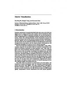
2 Related Work Visualization of DT-MRI and neuronal connectivity has taken many forms in the scientific visualization community. In this section we give an overview of some common approaches, but the reader is directed to the surveys by Margulies et al. [7] and Pfister et al. [8] for a more thorough treatment. Many approaches from vector- and tensorfield visualization, such as glyphs and streamlines, have been applied to the problem of connectivity visualization. Early tractography methods [5] were similar to streamline computations in fluid mechanics. Fibers are traced from a starting point by repeatedly stepping in the local direction of principal diffusion. However, visualization of the connectome by displaying streamlines or streamtubes is not practical due to the large number of streamlines required to represent whole brain connectivity. Fibers near the cortical surface of the brain occlude the inner structure, and the resulting image appears very cluttered, as seen in Figure (1). Volume rendered connectivity maps [9, 10] only display connectivity from a single seed point or region of interest as shown in Figure (1). Although GPU implementations permit exploration of the full dataset at interactive rates, it cannot give a comprehensive visualization of whole brain connectivity.
Fig. 1. Glyph-based visualization of white matter fiber orientation probabilities (left), volume rendered connectivity (middle), and neuronal fiber tracts (right) colored according to local direction. The glyphs convey the local structure of fiber orientations within a voxel but the global connectivity cannot be discerned. The volume rendering of connectivity shows only a small portion of the full connectivity matrix. The fiber tract visualization does convey global structure, but the clutter makes it difficult to visually follow individual fibers from end to end.
Connectivity matrices are square matrices Ci, j where the row and column indices correspond to either individual voxels or groups of voxels. A macroscale anatomical connectivity matrix can be assembled by registering an expert-labeled anatomical atlas to the diffusion weighted images. For each fiber path the endpoints can be mapped to
Graph-based visualization of neuronal connectivity
3
the regions-of-interest (ROIs) defined in the atlas. Each element of Ci, j then represents the connectivity of region i to region j. A connectivity graph corresponding to a connectivity matrix can be assembled by creating a node for each ROI, and computing node adjacency from Ci, j . Existing tools from network analysis and graph theory have been applied to this graph to determine its characteristics. As with other complex graphs, such as social networks, neuronal connectivity graphs are characterized by highly connected hub nodes and a small world topology (meaning there is a short path between every pair of nodes) [11]. Connectivity matrices are often visualized as an image with a colormap applied to the matrix elements. Permuting matrix rows and columns so that the ROIs are sorted from left to right results in a matrix that can readily yield inter- and intrahemispheric connectivity information. Sorted and unsorted connectivity matrices are shown in Figure (2). The sorted matrix can be split roughly (neglecting the brainstem) into quadrants: the upper-left is connectivity within the left hemisphere of the brain, the lower-right is connectivity within the right hemisphere, and the other two quadrants represent interhemispheric connectivity. Many approaches to improving or augmenting adjacency matrix visualization have been proposed [12–14], but the drawback shared by these methods is that the nodes lose locational meaning, which we wish to preserve.
Fig. 2. Connectivity matrix with rows and columns ordered arbitrarily (left), and with rows and columns sorted left to right by ROI position (middle). A 3D node-link diagram of the neuronal connectivity with anatomically embedded nodes (right). Note the occlusion and clutter due to the large number of edges, even though there are only 116 nodes.
Node-link diagrams are a popular approach to visualizing graphs and networks which may represent such diverse data as transportation routes and social relations. But even graphs of a moderate size can result in an unusable “hairball” visualization, such as in Figure (2, right). Nodes in graph based visualization may correspond to physical locations which should, in some applications, be preserved in the visualization because the relative positions of nodes provide valuable contextual information. A major problem with node-link visualizations is the visual clutter that occurs when many edges overlap. This can be avoided by using edge clustering and force-based edge bundling [15] to group edges and bend them around nodes. Previous approaches to connectivity visualization suffer from problems of visual clutter [16, 17] or loss of anatomical
4
Tim McGraw
context [18, 19]. Our goal in this work is to strike a balance between maintaining the spatial relations and anatomical meaning of the nodes of the connectivity graph while minimizing clutter due to the large number of edges.
3 Methods In this section we describe our visualization application which was implemented in Matlab. The input to our method is a connectivity matrix computed from diffusion MRI. Guided by psychological principles, we aim to simplify use of our application by reducing visual clutter and exploiting the user’s existing mental models. Overcrowded and disorganized displays have been shown to lead to decreased performance on visual search and recognition tasks [20]. We minimize visual clutter by separating inter- and intrahemispheric displays, and bundling edges. The existing mental models we build upon are the radiological conventions, such as standard imaging planes, and human anatomical knowledge. In the design of our application we eschewed a 3D approach to visualization since the degree of visual clutter and edge overlap is view dependent and therefore difficult to control. Node Layout Node locations were computed from the automated anatomical labeling (AAL) brain atlas which consists of 116 gray matter structures which were manually segmented from a human subject registered into a standard coordinate system [21]. A slice of the atlas is shown in Figure (3). We have further grouped the 116 labels into brain hemispheres (left, right) and regions roughly corresponding to brain lobes (shown in Figure (4)).
Fig. 3. A representative coronal slice of the AAL atlas with colored regions overlaid on T1weighted MRI (left), and partitioning of the sorted connectivity matrix (right). The brain is partitioned into left (L) and right (R) hemisphere, and medial (M) structures. The shaded blocks and unshaded blocks are visualized separately.
Anatomists and clinicians are trained to analyze medical images and identify structures by looking at images in 3 standard planes: axial, coronal and sagittal. We laid out
Graph-based visualization of neuronal connectivity
5
Hippocampus, Parahippocampus, Amygdala, Fusiform gyrus, Heschl gyrus, Superior temporal gyrus, Temporal pole: superior temporal Temporal Lobe gyrus, Middle temporal gyrus, Temporal pole: middle temporal gyrus, Inferior temporal gyrus Posterior Fossa Cerebellum, Vermis, Medulla, Midbrain, Pons Insula and Cingulate Gyri Insula, Cingulate gyrus (ant., mid, post.) Precentral gyrus, Superior frontal gyrus, Middle frontal gyrus, Inferior frontal gyrus, Rolandic operculum, Supplementary motor area, OlfacFrontal Lobe tory cortex, Gyrus rectus, Paracentral lobule Calcarine fissure and surrounding cortex, Cuneus, Lingual gyrus, OcOccipital Lobe cipital lobe (sup., mid. and inf.) Postcentral gyrus, Superior parietal gyrus,Inferior parietal gyrus, SupraParietal Lobe marginal gyrus, Angular gyrus, Precuneus Central Structures Caudate nucleus, Putamen, Pallidum, Thalamus
Fig. 4. Lobes and their constituent AAL labels. Most of the 116 AAL regions consist of left-right pairs.
our nodes in these standard planes by positioning each one at the centroid of its AAL atlas region and discarding one of the 3 coordinates of each node. Node positions were adjusted to prevent overlap using the method described by Misue et al. [22]. Nodes are drawn as color-coded circles with radius proportional to the degree (number of incident edges) of the node. Color is determined by which of the 7 lobes the node belongs to. The results we present in the next section use the coronal imaging plane for node layout. Edge Routing The connectivity matrix was thresholded to discard the lowest 1% of connectivity values, then edges consisting of line segments were created for each nonzero value in the connectivity matrix. Initially the edges consist of few segments (2-10, depending on length), but as the iterative process of bundling proceeds we refine the edges using midpoint subdivision. Edge bundling is performed in a manner similar to the process described by Holten and Van Wijk [15] with a few application specific differences. Edge bundling criteria are based on length compatibility, orientation, and visibility as in [15] but we add an anatomical compatibility criterion. We only bundle edges together if one or more of their endpoints is in the same lobe. We also add a small repulsion force between incompatible edges to try to separate them and avoid clutter. Block Partitioning of the Connectivity Matrix To achieve a similar connectivity grouping as the sorted matrix visualization in Figure (2), we display inter- and intrahemispherical connectivity separately. Interhemispheric fibers include some long pathways which are difficult to avoid when routing edges. By separating these fibers into their own visualization we reduce the problem to bipartite graph visualization. The connectivity matrix was sorted by node location from left to right and partitioned by the scheme shown in Figure (3). The shaded blocks of the connectivity matrix, representing intrahemispheric connectivity, are visualized together in a single view. The other two blocks which represent interhemispheric connections are shown in a separate
6
Tim McGraw
view. In our experiments, even with edge bundling, the long-range edges that cross the midline of the brain resulted in too much visual clutter. So interhemispheric connectivity is shown with a local scaling applied to node positions to shift them out of this region. The scaling applied to each hemisphere is given by the matrix product Tc−1 STc , where Tc translates the centroid of the hemisphere to the origin and S is a nonuniform scaling by 0.25 in the x-direction. Our application also supports interactive selection and highlighting of multiple lobes and atlas labels. For each selection the constituent nodes and all edges between them are shown in color. All other nodes and edges are drawn in a light gray color for context.
4 Results To generate the results shown in this section we used images from a publicly available dataset from the Neuroimaging Informatics Tools and Resources Clearinghouse (NITRC). Data for a set of 53 subjects in a cross-sectional Parkinson’s disease (PD) study was acquired. The dataset contains diffusion-weighted images (DWI) of 27 PD patients and 26 age, sex, and education-matched control subjects. The diffusion-weighted images were acquired with 120 unique gradient directions, b=1000 and b=2500 s/mm2 , and isotropic 2.4 mm3 voxels. The acquisition used a twice-refocused spin echo sequence in order to avoid distortions induced by eddy currents. The data were postprocessed to compensate for patient motion. Tractography and subsequent connectivity computation and visualization were performed on a Dell Optiplex workstation with a 3.4 GHz Intel Core i7-3770 CPU, and 8 GB RAM. Connectivity Matrix Computation From the diffusion weighted images we computed 4th order fiber orientation distribution tensors using the methods described by Weldeselassie et al. [23]. One million fiber tracts were generated by randomly seeding within the white matter and deterministically tracking until the fiber terminated. We use the AAL atlas to define 116 anatomical ROIs, so we initialize a 116 × 116 connectivity matrix to all zeroes (Ci, j = 0). The nearest AAL atlas region to each endpoint of the fiber was found and then the corresponding element of the connectivity matrix was incremented (Ci, j = Ci, j + 1). Since we have no basis on which to assume fiber directionality we make the connectivity matrix symmetric (C = C + CT ), resulting in an undirected connectivity graph. Control Group and Parkinson’s Group Visualization After computing C for each subject, the mean and variance of connectivity values for subjects in each group (PD and control) were computed. A node-link diagram of the resulting graph of 1842 edges with no partitioning or edge bundling is shown in Figure (5). Note the visual clutter near the midline where many edges cross as they pass between hemispheres. The mean control group intrahemispheric connectivity is shown using our proposed method in Figure (6). Since the interhemispheric connectivity is displayed separately the clutter near the midline in greatly reduced, and the edge bundling within each hemisphere makes the connectivity patterns more easily discerned. Large bundles of edges
Graph-based visualization of neuronal connectivity
7
Fig. 5. Visualization of the control group mean connectivity without matrix partitioning and edge bundling.
can be seen connecting to high degree nodes (represented with larger markers), emphasizing their importance as connectivity hubs. Left-right hemisphere asymmetry is clearly visible in this view, and is expected. This is due to many factors, including image noise, hard thresholding of connectivity values and lateralization of brain function. Functions such as speech and language are known to be controlled by the left cerebral hemisphere, especially the temporal and parietal lobes. Note that bilateral symmetry is not related to symmetry of the connectivity matrix (C = CT ). Control group interhemispheric connectivity visualization results are shown in Figure (7). Label and lobe selection by the user results in visual highlighting of connectivity. Although the node locations have been locally scaled, it is still possible to differentiate the nodes near the midline from the more lateral nodes. Parkinson’s disease is associated with impaired motor function and reduced cognitive performance. The disease is associated with dysfunction of the frontal lobe of the brain, and changes in functional connectivity have been observed in PD patients [24]. Connectivity differences between the PD and control groups were visualized by computing the absolute difference between connectivity matrices Cdiff = |CPD −Ccontrol |. An unpaired two-sample t-test at the 5% confidence level was performed for each pair of nodes (i, j). If the test did not reject the null hypothesis (that the mean connectivity in the groups is equal) then we set Cdiff(i, j) = 0. Visualization of this difference is shown in Figure (8). By selecting the nodes of the frontal lobe we can clearly see in Figure (9) that many of the connectivity differences between the PD and control group have connections to the frontal lobe.
5 Conclusion and Future Work In this work we have presented an approach to visualizing macroscale neuronal connectivity graphs which is designed to reduce user cognitive load by maintaining aqnatomical context. Visual clutter is reduced by partitioning the connectivity matrix into hemi-
8
Tim McGraw
Fig. 6. Visualization of the control group mean intrahemispherical connectivity. Lobes are colorcoded and connectivity weights are represented by edge thickness.
Fig. 7. Visualization of control group average interhemispherical connectivity for the whole brain (left), 3 selected lobes (middle) and a few selected nodes (right).
spheric blocks which are separately visualized using node-link diagrams with bundled edges. Hierarchical relations between brain hemispheres, lobes and regions-of-interest can be explored interactively, supporting coarse-to-fine investigation of connectivity. Examples of our technique were presented using data from a Parkinson’s disease study. Edge bundling revealed long-range connectivity patterns that are not visible in the naive node-link diagram or matrix visualization. In future work we plan to conduct a user study to assess which views and interactions permit experts to recognize meaningful connectivity patterns in the connectome.
References 1. Sporns, O., Tononi, G., K¨otter, R.: The human connectome: A structural description of the human brain. PLoS Computational Biology 1 (2005) e42
Graph-based visualization of neuronal connectivity
9
Fig. 8. Visualization of PD and control group connectivity differences. Statistically insignificant differences in connectivity are not shown.
2. Behrens, T.E., Sporns, O.: Human connectomics. Current Opinion in Neurobiology 22 (2012) 144–153 3. Micheva, K.D., Smith, S.J.: Array tomography: A new tool for imaging the molecular architecture and ultrastructure of neural circuits. Neuron 55 (2007) 25–36 4. Basser, P.J., Mattiello, J., LeBihan, D.: MR diffusion tensor spectroscopy and imaging. Biophysical Journal 66 (1994) 259 5. Basser, P.J., Pajevic, S., Pierpaoli, C., Duda, J., Aldroubi, A.: In vivo fiber tractography using DT-MRI data. Magnetic Resonance in Medicine 44 (2000) 625–632 6. Cammoun, L., Gigandet, X., Meskaldji, D., Thiran, J.P., Sporns, O., Do, K.Q., Maeder, P., Meuli, R., Hagmann, P.: Mapping the human connectome at multiple scales with diffusion spectrum MRI. Journal of Neuroscience Methods 203 (2012) 386–397 7. Margulies, D.S., B¨ottger, J., Watanabe, A., Gorgolewski, K.J.: Visualizing the human connectome. NeuroImage 80 (2013) 445–461 8. Pfister, H., Kaynig, V., Botha, C.P., Bruckner, S., Dercksen, V.J., Hege, H.C., Roerdink, J.B.: Visualization in connectomics. In: Scientific Visualization. Springer (2014) 221–245 9. McGraw, T., Nadar, M.: Stochastic DT-MRI connectivity mapping on the GPU. IEEE Transactions on Visualization and Computer Graphics 13 (2007) 1504–1511 10. McGraw, T., Herring, D.: High-order diffusion tensor connectivity mapping on the GPU. In: Advances in Visual Computing. Springer (2014) 396–405 11. Sporns, O.: The human connectome: A complex network. Annals of the New York Academy of Sciences 1224 (2011) 109–125 12. Dinkla, K., Westenberg, M.A., van Wijk, J.J.: Compressed adjacency matrices: Untangling gene regulatory networks. IEEE Transactions on Visualization and Computer Graphics 18 (2012) 2457–2466 13. Sheny, Z., Maz, K.L.: Path visualization for adjacency matrices. In: Proceedings of the 9th Joint Eurographics/IEEE VGTC conference on Visualization, Eurographics Association (2007) 83–90 14. Henry, N., Fekete, J.D., McGuffin, M.J.: Nodetrix: A hybrid visualization of social networks. IEEE Transactions on Visualization and Computer Graphics 13 (2007) 1302–1309 15. Holten, D., Van Wijk, J.J.: Force-directed edge bundling for graph visualization. Computer Graphics Forum 28 (2009) 983–990
10
Tim McGraw
Fig. 9. Visualization of PD and control group connectivity differences in the nodes belonging to the frontal lobe. The left frontal lobe, shown in the right side of the image by radiological convention, is seen to be the most affected lobe.
16. Bottger, J., Schafer, A., Lohmann, G., Villringer, A., Margulies, D.S.: Three-dimensional mean-shift edge bundling for the visualization of functional connectivity in the brain. IEEE Transactions on Visualization and Computer Graphics 20 (2014) 471–480 17. Li, K., Guo, L., Faraco, C., Zhu, D., Chen, H., Yuan, Y., Lv, J., Deng, F., Jiang, X., Zhang, T., et al.: Visual analytics of brain networks. NeuroImage 61 (2012) 82–97 18. Al-Awami, A., Beyer, J., Strobelt, H., Kasthuri, N., Lichtman, J., Pfister, H., Hadwiger, M.: Neurolines: A subway map metaphor for visualizing nanoscale neuronal connectivity. IEEE Transactions on Visualization and Computer Graphics (Proceedings IEEE InfoVis 2014) 20 (2014) 2369–2378 19. Irimia, A., Chambers, M.C., Torgerson, C.M., Van Horn, J.D.: Circular representation of human cortical networks for subject and population-level connectomic visualization. NeuroImage 60 (2012) 1340–1351 20. Rosenholtz, R., Li, Y., Nakano, L.: Measuring visual clutter. Journal of Vision 7 (2007) 1–22 21. Tzourio-Mazoyer, N., Landeau, B., Papathanassiou, D., Crivello, F., Etard, O., Delcroix, N., Mazoyer, B., Joliot, M.: Automated anatomical labeling of activations in SPM using a macroscopic anatomical parcellation of the MNI MRI single-subject brain. NeuroImage 15 (2002) 273–289 22. Misue, K., Eades, P., Lai, W., Sugiyama, K.: Layout adjustment and the mental map. Journal of Visual Languages and Computing 6 (1995) 183–210 23. Weldeselassie, Y.T., Barmpoutis, A., Stella Atkins, M.: Symmetric positive semi-definite Cartesian tensor fiber orientation distributions (CT-FOD). Medical Image Analysis 16 (2012) 1121–1129 24. Baggio, H.C., Sala-Llonch, R., Segura, B., Marti, M.J., Valldeoriola, F., Compta, Y., Tolosa, E., Junqu´e, C.: Functional brain networks and cognitive deficits in Parkinson’s disease. Human Brain Mapping 35 (2014) 4620–4634