1. 2. 3. 4. (c). Figure 1: (a) An undirected graph. (b) A clique decomposition of (a).
(c) 5 2-cliques, or 2 ... For example, in Fig.2a we show the Political Books links.
Graph Clustering, Clique Matrices and Constrained Covariances∗ David Barber Department of Computer Science, University College London
4
3
6
1
2
5
(a)
4
3
3
6
1
2
2
5
(b)
2 1
4 3 (c)
Figure 1: (a) An undirected graph. (b) A clique decomposition of (a). (c) 5 2-cliques, or 2 3-cliques. An interesting analysis is to break an undirected graph, Fig.1a, into well-connected clusters of nodes, Fig.1b. Forming such a ‘decomposition’ could be found by recursively identifying the largest clique in the graph1 . Whilst such a ‘greedy’ recursive approach is feasible, it depends on finding maximal cliques, itself an NP-hard problem. Furthermore, this requirement may be also be too strict since, provided that only a small number of links in an ‘almost clique’ are missing, this may be considered a sufficiently well-connected group of nodes to cluster them. Incidence and Clique Matrices The incidence matrix Zinc describes the adjacency structure: For each link ij, form a column of Zinc with zeros except for a 1 in the ith and j th row. The column ordering is arbitrary. For example, for Fig.1c 1
Zinc
1 = 0 0
1 0 1 0
0 1 1 0
0 1 0 1
0 0 , 1 1
1
1 Z= 1 0
The incidence matrix has the following remarkable property: � T A = H Zinc Zinc
0 1 1 1
(1)
(2)
where A is the adjacency matrix, including self-connections, and [H(M )]ij = 1 if Mij > 0 and is 0 otherwise (H(·) is the element-wise Heaviside step function). One may view Zinc as a decomposition into two-cliques, since each column contains only two entries. Another decomposition of Fig. 1c is into two (maximal) cliques (123), (234). The matrix Z � in Eq. (1) also satisfies A = H ZZ T . We introduce the terminology clique matrix for Z since each column expresses which nodes form a clique. (The incidence matrix is special case, namely a 2-clique matrix). The number of columns of the clique matrix is the number of cliques, and each column describes the clique. To perform clustering, we would like to find the smallest number of maximally-sized-cliques. That is, Z should have a small number of columns. Constrained Relational Covariances Clique matrices solve the following problem in Relational Machine Learning : Given an adjacency matrix A, find a covariance matrix that contains zeros where A is zero. For example, in Fig.2a we show the Political Books links (from Valdis Krebs). In recent works on Relational Learning (e.g. Silva, Chu, Ghahramani, NIPS 2007), a model of covariances of these relations is required, with zero-covariance where A is zero. Since, by construction, A = H(ZZ T ), then ZZ T is a covariance matrix, with zeros where A has zeros. Hence, by forming U to be zero where Z is zero, and choosing any values for the remaining elements, C = U U T is a covariance matrix. The incidence matrix is one way to do this, but over-parameterised. A clique matrix offers a more parsimonious parameterisation2 . The clique-matrix formalism also provides a route to parameterising diffusion kernels (eg. Tsuda and Noble, Bioinformatics 20, 2004). ∗ An
early version of this work was presented at the 6th Slovenian International Conference on Graph Theory, Bled, 2007. V 0 for the initial vertex set and C 0 as the largest clique of the graph on V 0 . Then remove those nodes of the largest clique not �� connected with the rest of the graph. More formally, recursively identify the largest clique on the remaining nodes V i+1 ≡ V i \ C i \ V i ∩ C i . 2 Using β = 10, we found Z in Fig.2c which satisfies A = H(ZZ T ), solving the constraint. Bigger clusters can be found using a smaller β, if desired. This would be at the expense of clusters not being fully-connected, and wouldn’t perfectly solve the constraint problem. 1 Write
1
40 20
20
20
20
40
40
40
40
60
60
60
60
80
80
80
80
100
100
100
100
35 30 25 20 15 10
20
40
60
80
100
100
(a)
200
300
400
20
(b)
40
60
80
100
120
140
5 0 20
(c)
40
60
80
100
(d)
Figure 2: (a) Adjacency matrix of 105 Political Books (black=1). (b) Incidence Matrix: 882 non-zero entries. (c) Clique matrix: 521 non-zero entries. (d) Sampled Covariance, generated from (c) with constraints implied by (a) obeyed. Finding Probabilistic Approximate Clique Decompositions To find ‘well-connected’ clusters, we relax the problem so that the absence of links are viewed as statistical fluctuations away from a perfect clique. Given a clique matrix Z, we desire that the higher the overlap between rows zi and zj is, the greater the probability of a link between i and j. We express this using � p(i ∼ j|Z) = σ zi zjT ,
σ(x) ≡
1 1+
(3)
eβ(0.5−x)
where β controls the steepness of the function. Absent links contribute p(i 6∼ j|Z) = 1 − p(i ∼ j|Z). Under Eq. (3), if zi and zj have at least one ‘1’ in the same position, zi zjT − 0.5 > 0 and p(i ∼ j) is high. Assuming each element of A is �Q �� Q T sampled independently the likelihood is p(A|Z) = i∼j σ zi zjT . For small β, subsets that would i6∼j 1 − σ zi zj be cliques, if it were not for a small number of missing links, form a cluster. To bias Z to have a small number of cliques, we reparameterise Z as a set of column vectors z: Z˜ = (α1 z1 , . . . , αCmax zCmax )
(4)
where αc ∈ {0, 1} are indicators. We define a Beta-Bernoulli process prior on α to encourage a small number of α′ s to be used. The resulting posterior p(α, Z|A) is intractable and requires approximation. We therefore implemented a collapsed Variational Bayes approximation, including additional Mean-Field Theory assumptions. In Fig. 3 we examined a ‘difficult’ DIMACS challenge problem which hides a single large clique of size 12 amongst many smaller cliques. Our algorithm successfully found a complete description of all clusters in the graph. Summary and Outlook We consider graph clustering by extending the incidence matrix formalism to more general clique-matrices. Embedded within a statistical framework, we can decompose a graph into clusters, using a parameter to control how ‘perfect’ the cliques should be. To encourage large cliques to be discovered, we use a Beta-Bernoulli prior on the columns in the clique matrix. Formally the resulting inference problem is hard, but can be approximated using, for example, Variational Bayes. Using clique matrices, we showed how to solve problems in Relational Machine Learning requiring constrained covariance matrices. The same ideas can be applied to (diffusion) kernel-learning. In addition, we successfully found a complete clique decomposition of a ‘difficult’ DIMACS graph which, by construction, is not amenable to some standard recursive MAX-CLIQUE approximations. We’ve additionally applied our technique to cluster gene-expression profiles and find large well-connected clusters in social networks. In the future we will investigate alternative inference approximations in order to scale up to larger systems. Our c-code implementation is available on request. 8 7 50
50
100
100
150
150
6 5 4 3 2 1
200
50
100
(a)
150
200
200
200
400
600
(b)
800
1000
0
1 2 3 4 5 6 7 8 9 10 11 12
(c)
Figure 3: (a) Adj. matrix for the DIMACS brock200-2 MAX-CLIQUE challenge. (b) Clique Matrix. (c) Log2 -histogram of clique-sizes(+1) in the Clique Matrix; correctly solves MAX-CLIQUE (12) as well as identifying all remaining clusters. 2