Graph Coding and Connectivity Compression Martin Isenburg†
Jack Snoeyink‡
University of North Carolina at Chapel Hill
Abstract This paper looks at the theoretic roots of current connectivity compression schemes to establish a visual framework within which the differences and similarities of various scheme become intuitive. We show the intimate connections between the classic work on planar graph coding by Turan and recent schemes, such as Edgebreaker, Face Fixer, and the optimal coding by method of Poulalhon and Schaefer. Furthermore we fit Touma and Gotsman’s valence coder into this classification. This helps to explain what information is hidden in the "split offsets" and suggests a strategy for doing valence coding without using offsets. Other results are an elegant method for reverse decoding of meshes encoded with Poulalhon and Schaefer’s optimal coder, and the insight that the classic Keeler and Westbrook method and the Edgebreaker scheme are really the same algorithm for the case of encoding planar triangulations. Finally, we conjecture that (a) optimal encodings are never streamable and (b) encodings that avoid offsets necessarily result in uncoherent mesh layouts.
1. Introduction A polygon mesh is the most widely used primitive for representing three-dimensional geometric models. Such polygon meshes consists of mesh geometry and mesh connectivity, the first describing the positions in 3D space and the latter describing how to connect these positions together to form polygons that describe a surface. Typically there are also mesh properties such as texture coordinates, vertex normals, or material attributes that describe the visual appearance of the mesh at rendering time. The standard representation of a polygon mesh uses an array of floats to specify the positions and an array of integers containing indices into the position array to specify the polygons. A similar scheme is used to specify the various properties and how they are attached to the mesh. For large and detailed models this representation results in files of substantial size, which makes their storage expensive and their transmission slow. The need for more compact representations has motivated researchers to develop efficient mesh compression schemes. †
[email protected] ‡
[email protected]
A typical mesh compressor has different components for dealing with the different types of mesh data. Compression of mesh geometry is usually lossy because the original floating point positions are initially quantized onto a uniform grid. Compression of mesh connectivity is generally considered lossless as the incidences between the vertices are recovered exactly. However, neither the original values of the indices (e.g. the ordering of vertices) nor the original order of the indices in the index array (e.g. the ordering and rotation of triangles) are preserved. Overall, the research efforts in mesh compression have focused mostly on efficient encodings for mesh connectivity 10, 52, 53, 40, 16, 44, 35, 23, 3, 24, 36, 48, 2, 19, 32 . There are several reasons for this: First, this is where the largest gains are possible, second, the combinatorical nature of the problem has an irresistable appeal to researchers, and third, the connectivity coder is the core component of the compression engine and usually drives the compression of geometry 10, 52, 53, 30, 20, 37 , of properties 10, 51, 3, 27 , and of how properties are attached to the mesh 51, 24, 26 . Connectivity compression has its roots in graph theory where its foundations were laid 55, 54, 31 . It was first brought to the computer graphics community to speed up the rendering of triangle meshes 10 , was then improved for maxi-
2
Isenburg and Snoeyink / Graph Coding and Connectivity Compression
mum compression 52, 53, 40, 16, 44 and later generalized for nontriangular meshes 39, 24, 36, 19, 32 . It has traveled since into the field of computational geometry where the focus shifted towards algorithmic efficiency 45, 25 and guaranteed bounds on the code size 34, 48 . Its theoretic origins were revived by the quest for provable optimal encodings for mesh connectity 2, 32, 11 and planar graphs 17 with Poulalhon and Schaefer’s optimal method 42 finally joining the two communities. Recently, connectivity compression continued its voyage into the areas of out-of-core algorithms and stream processing 21, 22 where not only compactness but also streamability becomes an objective for the encoding. In this paper we go back to the roots of graph coding and establish a visual framework which can intuitively explain the differences and similarities between various scheme. We show the intimate connections between the classic work by Turan 54 and recent schemes, such as Edgebreaker 44 , Face Fixer 24 , and the optimal coding by method by Poulalhon and Schaefer 42 . We mostly follow the timeline of the research that starts with Tutte’s results on the enumeration of triangulations 55 and the coding of planar graphs with spanning trees 54 . Once these ideas are brought to the graphics community 10, 52 the coding strategy shifts away from explicit spanning tree coding 54, 31, 52 to more elegant region-growing approaches 53, 16, 39, 44 that are later generalized to the polygonal case 24, 36, 19, 32 . While these schemes have been classified into facebased 16, 44 , edge-based 39, 24 , and vertex-based 53, 23 schemes, there has been little intuitive understanding about there differences. We characterize their differences by fitting them into the same visual framework, which makes clear in which way these schemes are similar to the early work by Turan 54 and in which way they improve on it. We form a second, parallel classification of these schemes into one-pass 53, 16, 39 and multi-pass 52, 44, 24 coders. This divides the existing body of compression schemes into those that can be used out-of-core 21 and those that can not. For the main part, we focus on the case of fully triangular meshes without holes or handles. This class of meshes is homeomorphic to maximal planar graphs or planar triangulations. We do not address the compression of geometry or properties. Neither do we consider progressive compression methods 50, 8, 41, 1 , which encode a mesh incrementally at multiple resolutions, nor shape compression methods 33, 12, 49 , which do not encode a particular mesh, but a highly regular remesh of its geometric shape.
cycle is called an half-edge. It has an orientation that is determined by the order of the vertices on either side. Around each vertex we find one or more oriented rings of faces and edges. An edge is manifold if it is either shared by two faces of opposite orientation or used only by one face, in which case it is also a border edge. An edge shared by more than two faces is non-manifold. A vertex is manifold if its incident edges are manifold and connected across faces into a single ring. Topologically, a mesh is a graph embedded in a 2manifold surface in which each point has a neighborhood that is homeomorphic to a disk or a half-disk. Points with half-disk neighborhoods are on the boundary. A mesh has genus g if one can remove up to g closed loops without disconnecting the underlying surface; such a surface is topologically equivalent to a sphere with g handles. A mesh is simple if it has no handles and no border edges. Euler’s relation says that a graph embedded on a sphere having f faces, e edges, and v vertices satisfies f − e + v = 2. When all faces have at least three sides, we know that f ≤ 2v − 4 and e ≤ 3v − 6, with equality if an only if all faces are triangles. For a mesh with g handles (genus g) the relation becomes f − e + v = 2 − 2g and the bounds on faces and edges increase correspondingly. 3. Coding Mesh Connectivity The standard approach that represents the connectivity of a mesh with a list of vertex indices requires at least kn log2 n bits, where n is the total number of vertices and k is the average number of times each vertex is indexed. For a simple triangular mesh, Euler’s relation tells us that k will be about 6. For typical non-triangular meshes that contain a mix of polygons dominated by quadrangles, k tends to be around 4. The problem with this representation is that the space requirements increase super-linearly with the number of vertices, since log2 n bits are needed to index a vertex in an array of n vertices.
2. Preliminaries
Efficiently encoding mesh connectivity has been subject of intense research and many techniques have been proposed. Initially most of these schemes were designed for fully triangulated meshes 10, 52, 53, 40, 16, 44, 23, 3, 18, 48, 2 , but more recent approaches 35, 24, 36, 32, 19 also handle arbitrary polygonal input. These schemes do not attempt to code the vertex indices directly—instead they only code the connectivity graph of the mesh. The mapping from graph nodes to vertex positions is then established though an agreed upon ordering derived from the connectivity graph.
A triangle mesh or a polygon mesh is a collection of triangular or polygonal faces that intersect only along shared edges and vertices. Around each face we find an oriented cycle of vertices and edges. Each appearance of a vertex in this cycle is called a corner. Each appearance of an edge in this
Hence, mesh connectivity can be compressed by coding the connectivity graph and by changing the order in which the vertex positions are stored. They are arranged in the order in which their corresponding graph node is encountered during some deterministic graph traversal. Since encoding and
Isenburg and Snoeyink / Graph Coding and Connectivity Compression start sym + – ( )
# code v-1 00 v-1 01 2v-5 10 2v-5 11
sym
6
)
( )
+ – (
)
+ –
+
# code v-1 00 v-1 01 2v-5 1
7
)
(
+
+
+–
)
( 4
1
– ( (
+ )
(
– (
5
+ (
9
(
4
(
+
+ ) 8
9
start
( (
–
–
–
+
–
+ )
9
7
1
5
(
+
) )
– –
–
(
(
4
(
(
6
7
6v-9 bits 12v-14 bits
3
(
8
) (
– +
9
(
(
+
(
+
2
)
3
+
3
)
–
(
(
2
–
8
( ( –
4
7
–
Figure 1: To code planar graphs Turan performs a walk around a vertex spanning tree during which he records four different symbols, +, -, (, and ). It’s not too hard to see that for fully triangulated graphs we may omit either all opening or all closing brackets. The respective other brackets can be derived from the fact that all faces are triangular. Turan’s illustrates his method by “pulling open” the graph along the path around the vertex spanning tree. We will use this as a visual framework that illustrates how recent connectivity coders manage to encode the same information with fewer bits.
decoding of the connectivity graph also requires a traversal, the positions are often reordered as dictated by this encoding/decoding process. This reduces the number of bits needed for storing mesh connectivity to whatever is required to code the connectivity graph. This is good news: the connectivity graph of a polygon mesh with sphere topology is homeomorphic to a planar graph. It well known that such graphs can be coded with a constant number of bits per vertex 54 and exact enumerations exist 55, 56 . If a polygon meshes has handles (i.e. has non-zero genus) its connectivity graph is not planar. Coding such a graph adds a logarithmic number of bits per handle 52 , but most meshes have only a very small number of handles. Unfortunately the connectivity can only be coded this way for manifold polygon meshes. One would expect polygonal surfaces that describe solid objects to have this property. However, non-manifoldness is often introduced by mistake when converting from other surface representations. Also hand-authored content is frequently non-manifold, especially if the artist tried to optimize the mesh (e.g. minimize its vertex count). The problem of efficiently coding non-manifold graphs is hard and there are no optimal solutions yet. Most schemes either require the input mesh to be manifold or use a preprocessing step that cuts non-manifold meshes into manifold pieces 14 . Cutting a non-manifold mesh replicates all vertices that sit along a cut. Since it is generally not acceptable to modify a mesh during compression, the coder needs to describe how to stitch the mesh pieces back together. Guéziec et al. 13 report how to do this in an efficient manner and Isen-
burg 19 implements a simpler stitching scheme at the expense of less compression. Although this scheme was originally intended only for typical meshes with few non-manifold vertices, it has also proved sufficient for highly non-manifold models 21 . 4. Coding Planar Graphs Tutte’s early enumeration results 55, 56 imply that an unlabeled planar graph can be represented with a constant number of 3.24 bits per vertex. Similarly, Itai and Rodeh 29 prove that a triangular graph with v vertices may be represented by 4v bits. However, these existance proofs do not provide us with an effective procedure to construct such a representation. Turan 54 is the first to report an efficient algorithm for encoding planar graphs with a constant number of bits. A planar graph with v vertices, f faces, and e edges can be partitioned into two dual spanning trees. One tree spans the vertices and has v − 1 edges, while its dual spans the faces and has f − 1 edges. Summing these edge counts results in Euler’s relation e = (v − 1) + ( f − 1) for planar graphs. Turan observed that the partition into dual spanning trees can be used to encode planar graphs and reported an encoding that uses 4 bits per edge (bpe) for general planar graphs. Applying his method to fully triangulated graphs results in an encoding that uses 12 bits per vertex (bpv). This bit-rate, which is often quoted in literature, is unnecessarily inflated. We can improve the Turan’s bit-rate to 6 bpv simply by using of the fact that every face is a triangle. The encoding method of Turan walks around a vertex
4
Isenburg and Snoeyink / Graph Coding and Connectivity Compression
spanning tree and records four different symbols as illustrated in Figure 1. Two symbols “+” and “–” describe walking down and up the edges of the vertex spanning tree. Two symbols “(” and “)” describe walking across edges that are not part of the vertex spanning tree for the first and for the second time. This information encodes both spanning trees and is sufficient to reconstruct the original graph. There are v − 1 symbols each of type “+” and “–”, one pair for each edge of the vertex spanning tree. There are e − v + 1 symbols each of type “(” and “)”, one pair for each edge not part of the vertex spanning tree. Coding each symbol with 2 bits leads to an encoding for planar graphs that uses 4v − 4 + 4e − 4v + 4 = 4e bits. 6
C C C
R E C
6
7
L
C
C
R
7
C
5
18 19
9
C
5
L
E
R
4 C
S
R E R R C C
R
2
3
C
R C
1
C R
7
S
C R
17
C
5
6 C
8
9
10
S 11
C
8
4
15
16
4
11
12
17
R
3
13
R
14
3
3
10 8
16
C
R 13
3
3
14
9
L
12
2
18
E
E
15
19
1 1
2
Figure 2: To code triangulated planar graphs Keeler and Westbrook construct a triangle spanning using a topological depth-first sort. The nodes of this tree, which they classify as types 1 to 5, are identical to the five cases C, L, E, R, and S of the Edgebreaker encoding. The straight-forward application of Turan’s method to fully triangulated graphs where e = 3v − 6 results in an encoding that uses 12v − 18 bits. However, when every face is a triangle, we only need to include either all “(” or all “)” symbols in the code. The respective other can be omitted as it can be derived with some simple book-keeping. This observation leads to a much tighter bound of 6v − 9 bits by encoding the v − 1 occurances of “+” and “–” with two bits and the 2v − 5 occurances of either “(” or “)” with one bit. Given the choice about which of the two bracket types to encode we would argue for keeping the closing brackets. While this makes no difference to the implementation of the encoding algorithm, it leads to a slightly more elegant implementation of the decoder. Using opening brackets requires the decoder to check whether another triangle is to be formed after each non-bracket symbol and also after each formed triangle. When using closing brackets, however, we simply form one triangle whenever the decoder reaches a bracket symbol by connecting back to the vertex that is reached by going two steps backwards along the last two edges. Improving on Turan’s work, Keeler and Westbrook re-
port a 3.58 bpe encoding for general planar graphs, which they specialize to a 4.6 bpv encoding if the graph is triangulated 31 . Again, a small oversight on the author’s part results in the latter bit-rate being unnecessarily inflated. We can improve their bit-rate to 4 bpv simply by changing their mapping from symbols to bit codes. This oversight has also helped obscure the intimite similarities between Keeler and Westbrook’s method 31 and Rossignac’s Edgebreaker scheme 44 . For the case of encoding planar triangulations these schemes perform exactly the same traversal and distinguish exactly the same five cases. The main difference between them is how they map each case to a bit code. The encoding method of Keeler and Westbrook and its equivalence to the Edgebreaker method are illustrated in Figure 2. Keeler and Westbrook construct a triangle spanning tree using a topological depth-first sort in the dual graph. It is the determinism with which this triangle spanning tree— and the corresponding vertex spanning tree—is created that allows them to improve on the bit-rates of Turan’s method, which assumes no particular vertex spanning tree. Each dual edge that is not part of the triangle spanning tree crosses a primal edge that is part of the vertex spanning tree. It connects two nodes of the triangle spanning tree and one of these nodes will be an ancestor of the other. Keeler and Westbook declare the ancestor node to have a missing child where this dual edge connects (illustrated by a red dot in the figure) and attach a leaf node to where this edge connects at the other end (illustrated by a green dot). The resulting tree has only five different types of non-leaf nodes and is encoded through a pre-order traversal that maps them to different bitcodes. The type of a non-leaf depends on its parenthood. A non-leaf node can either have:
1. 2. 3. 4. 5.
two non-leaf children (S). a non-leaf left child and a missing right child (C). a non-leaf left child and a leaf right child (L). a leaf left child and a non-leaf right child (R). two leaf children (E).
As indicated, these nodes are identical to the five cases distinguished in the Edgebreaker encoding. Keller and Westbrook observe that half of all nodes will have leaves, meaning will be of type L, R, and E. They devise a mapping from node types to bit codes that represents C as 00, S as 01 and either of L, R, or E with 1. To that encoding they append a bitstring that distinguishes between L, R, and E using log2 (3) bits each. The total results in the reported bitrate of 4.6 bpv. Would the authors have instead noticed that half of all nodes have a missing child, meaning are of type 2, they could have easily formulated the more efficient 4 bpv encoding that was therefore not discovered until Rossingac’s much more elegant formulation of this algorithm termed Edgebreaker 44 .
Isenburg and Snoeyink / Graph Coding and Connectivity Compression processed region
5
boundary free edge
unprocessed region
focus
T
T
R
T
R
Figure 3: The three different approaches to connectivity coding by region growing: edgebased (top), face-based (middle), and vertexbased (bottom). Every iteration of the edgebased coder processes the free edge and describes its adjacency relation to the active boundary. Similarly every iteration of the face-based coder processes the free face and describes the adjacency relation. For both coders these descriptions specify how the active boundary is updated. When the vertexbased coder processes a face, it only needs to describe what happens at the free vertex of this face to specify the boundary update.
processed region
boundary free face
unprocessed region
focus
C
R
R
--
--
end slot start slot free vertex
boundary slots
V5
5. Compressing Mesh Connectivity Taubin and Rossignac 52 introduced these graph coding techniques to the graphics community for compressing triangle meshes. Like Turan they encode triangular connectivity using a pair of spanning trees, but unlike Turan they code the two trees seperately. When using run-length coding, this results in bit-rates of around 4 bpv in practice but leads to no guaranteed bounds. Rossignac 43 later pointed out that using a standard 2 bit per node encoding for each of the two trees also guarantees a 6 bpv bound. Most importantly, their work showed how to integrate topological surgery into the encoding process for dealing with non-planar connectivity graphs. This is done by identifying pairs of triangles in the triangle spanning tree that are glued together to recreate a handle, which can always be done with O(log2 (v)) bits per handle. Since most meshes have only a small number of handles, no efforts have been directed at establishing tighter bounds. Recently proposed encoding schemes 53, 16, 40, 44, 24 do not explicitly construct the two spanning trees. Instead they traverse the connectivity graph using a region growing approach during which they produce a symbol stream that implicitely encodes both trees in an interleaved fashion. These schemes maintain a set of boundary loops that separate a single processed region from all unprocessed regions. The edges and vertices on the boundary are called boundary edges and boundary vertices and they are considered visited. Each boundary encloses an region containing unprocessed edges, faces, and vertices. If the connectivity graph has handles, these boundaries can be nested, in which case an unprocessed region is enclosed by more than one boundary. Each boundary has a distinguished edge or vertex called the focus. These algorithms work on the focus of the active boundary, while all other boundaries are kept in a stack.
focus (widened)
At each step, these algorithms describe how the unprocessed mesh element at the focus is adjacent to the active boundary. Depending on the graph elements that the description of this update can be thought of as being associated with, these schemes have been classified as edge-based, face-based, and vertex-based. Only for a non-zero genus connectivity there will be one situation per handle in which this description involves a boundary from the stack. Face-based schemes 16, 44 describe all boundary updates per face. The boundaries are loops of edges that separate the region of processed faces from the rest. Each iteration grows the processed region by the face adjacent to the focus of the active boundary. It is adjacent to the active boundary in one of five ways. Edgebreaker 44 describes the boundary updates corresponding to these five configurations using the symbols C, R, L, S, or E. The Cut-Border Machine 16 associates an additional split offset with each S that—from a coding point of view—is redundant but allows streaming compression and decompression. A number of guaranteed worst-case bounds for coding triangular connectivity have been established based on Edgebreaker’s CLERS 34, 48, 15 . Edge-based schemes 40, 24 describe all boundary updates per edge. The boundaries are loops of half-edges that separate the region of processed edges from the rest. Each iteration grows the processed region by the edge adjacent to the focus of the active boundary. It is either adjacent to an unprocessed triangle or to the active boundary in one of four different ways. Face Fixer 18, 24 describes the boundary updates corresponding to these five configurations using the symbols T , R, L, S, or E. The Dual Graph method 39 does the same but associates an additional split offset with each symbol that represents a distance in number of edges along the boundary. Vertex-based schemes 53 describe all boundary updates per vertex. The boundaries are loops of edges that separate
6
Isenburg and Snoeyink / Graph Coding and Connectivity Compression
sym C LE RS
# code v-3 1 v-2 0 x
–
– –
8 18 R
19 E
x
+
6
12
1
+
4v-9 bits
–
C12
3
3
–
E15
+ 5
S11
16 L
–
R14
1
1
L 29
6
17 C
–
–
R 13
– R
– R
8
T27
L 22
T25
21R
T 23
15T
– E 30 –
6
T 20
9
T16
– –
19 R 10
17 R
14 T
7
code
5v-8 bits
5
T18
#
1 T 2v-5 LE v-1 0 x x RS
–
12
24 T
1
10
9
sym
+
6
26
28
–
6
+
11
9C
R10
+ 8
R7
+
5 6
7
19
5
18
+
– 2
3C
5
+
17
start R 4
C 2
C
1
C
4
10
+
11
3
+
6T
6
+
3T
5
+
1
+
5
12
3
3
9
5
2
R
– 8
1T
2T
4
10
4
+
start
T4
5
+
7
7
6
9
R–
9
7T
7
6
+
T8 8
8
R– 4
10 T
+
– 7
6C
13
1
4
8C
11
11 T
–
1
T 12
+
11
7
+
7 9
+
+
10
3
8 16 9
15 11 12 14 13
10
4
26 27 25 28 29 24 23
10 30
8
11
3
4
2 2
1
start 44
5
20 16 18 19 4 17 3 2
14
12
2 1
21 22 15
3
11
6
13 1
24
Figure 4: The Edgebreaker (left) and the Face Fixer (right) algorithms traverse mesh triangles in the same depth-first order thereby constructing the same two spanning trees (middle). Because of their deterministic construction the labeling of these spanning trees can be compressed more efficiently than Turan’s generic trees.
the region of processed faces from the rest. Furthermore, they store for every boundary vertex the number of free degrees or slots, which are unprocessed edges incident to the respective vertex. Each iteration grows the processed region by the face adjacent to the widened focus of the active boundary. The focus often needs to be widened such that there is a start slot and an end slot for the face. Only if the processed face has a free vertex that is not part of the widened focus, the boundary update needs to be described. Two scenarios are possible: either the free vertex has not been visited, in which case its degree is recorded, or is has been visited, in which case a distance in slots along the active boundary is recorded and the active boundary is split. A important classification for practical purposes is whether an encoding allows a one-pass replay of the encoding process during decoding or whether it performs multipass decompression. We return to that in the last section. Now we want to focus our attention on Figure 4. Just like Turan’s original method both Edgebreaker 44 , a facebased scheme that does not use offsets, and Face Fixer 24 , an edge-based scheme that does not use offsets, label the two spanning trees. They manage to do so using fewer bits because they use spanning trees with certain properties (e.g. that are result of systematically traversing the graph in a depth-first manner). The same can be said about Keeler and Westbrook’s method 31 since the symbols it produces have the same meaning as those produced by Edgebreaker. Each Edgebreaker label C corresponds to a “+” and marks an edge of the triangle spanning tree. Labels R and L correspond to a “–” and mark an edge of the triangle spanning tree. S marks two edges of the triangle spanning tree and E corresponds to two “–”. Marking the edges of the triangle
spanning tree may be thought of corresponding to either an opening or a closing bracket. There are two reason why the Edgebreaker labels allow a tighter bound on the code size than the Turan symbols: First, each of the five labels encodes a pair of Turan symbols, which—encoded independently— could form nine different combinations. Second, each C label pairs a “+” symbol with a bracket, which means that half of all labels are of type C. Note that the up and down labels “+” and “–” around the vertex spanning tree correspond exactly to the zip-directions used in the Wrap&Zip decoding method for Edgebreaker 45 Each Face Fixer label T marks an edge of the triangle spanning tree. Again, marking the edges of the triangle spanning tree may be thought of corresponding to either an opening or a closing bracket. Note that the original paper 24 uses labels F3 , F4 , F5 , ... in place of the T labels we use here. We follow the notation from 18 and write T instead of F3 because all our faces are triangles. Labels R, L, S, and E correspond to nested pairs of symbols “+” and “–”. The reason that the Face Fixer labels allow a tighter bound on the code size than the Turan symbols is that pairs of “+” and “–” can be encoded with 3 bits whereas encoding them independently requires two bits per symbols or 4 bits per pair. 6. Optimal coding of planar graphs The field of graph theory has recently seen new efforts towards optimal coding of planar graphs 17, 7 . All these schemes make use of specially ordered spanning trees inspired by the work of Schnyder 47 . Poulahon and Schaeffer 42 finally show that a particular Schnyder decomposition of a triangulation into three spanning trees can be used for optimal coding.
Isenburg and Snoeyink / Graph Coding and Connectivity Compression
v0
sym
7
+ –
+
# code v-1 1 v-1 0 2v-5 0
7
v0 7
+
v1
4
5
+
+
2
3
6
+
–
2
4
8
l2
2 3
8 5
3
8
13
14
12 16 10
5
1
15
17
9 15 10
–
9
–
19
12
12
11
18
10
start
12
–
10
6
13
14
+ 2
v2
+
8
16
11
v1
– 17
3 1
4
18
+
7
9
5
5
6
4
v0 –
4
1
6
7
11
+
1 6
–
19
7
6
l2
v1
20
–
~ 3.24…bpv
start
v2
1
5
9 12
+
11
–
9
6
+
–
–
Figure 5: Poulahon and Schaeffer construct a very particular vertex spanning tree. It has the property that when we walk around it we cross at each node exactly two triangle spanning tree edges for the second time. The visualization on the right shows that this corresponds to a Turan-style labeling that uses closing brackets. Note that the original algorithm 42 walks the opposite direction which corresponds to the use of opening brackets.
Starting from a triangulation with an embedded maximal realizer † Poulahon and Schaeffer construct a very particular vertex spanning tree that is shown in Figure 5. This vertex spanning tree has the property that a counterclockwise walk that starts at the root crosses at each node (but the first three) exactly two non-spanning tree edges for the second time. The original algorithm suggests to walk in clockwise direction with the similar result that at each node (but the first three) exactly two non-spanning tree edges are crossed for the first time. The right illustration in Figure 5 shows that this corresponds to a Turan-style labeling that uses only closing brackets (or only opening brackets when using the walk direction employed in the original algorithm). The reason that Poulahon and Schaeffer’s encoding gives a tighter bound on the code size than the Turan symbols is that they manage to get away using just a single bit for each symbol “+”, “–”, “)”. This is because their algorithm knows that in this particular spanning tree, the first and the second occurance of a zero bit at a node corresponds to a closing bracket, whereas the third zero bit must signal the “–”. Therefore the one bit can be reserved to express the “–” symbols. The resulting bit string contains 4n bits of which n bits are ones while the the remaining 3n bits are zero. There are 4novern different such strings and they can be encoded in linear time into a representation that uses only 246n/27 or 3.24n bits 5 . This coincides with the optimal worst-case † An intuitive algorithm for constructing the maximal realizer of a triangulation is described in Enno Brehm’s Diploma Thesis 6 .
bounds for encoding planar triangulation that can be derived from Tutte’s enumeration work 55 . Hence, because Poulahon and Schaeffer’s choice in vertex spanning tree is even more particular than that of Edgebreaker or Face Fixer, they are able to improve the worst-case bound for the code-size to the optimum of 3.24 bpv. 7. Coding with Vertex Degrees In this section we investigate how the vertex-based coding scheme by Touma and Gotsman 53 fits into all this. This is especially interesting given recent claims that valence coding is optimal—at least under the assumption that some part of the code, namely the split operations and their associated offsets, have no significant impact on the total code size. If no splits occur, the encoding is merely a sequence containing the degree of every vertex. A result by Alliez and Desbrun 2 gave reason to believe that the entropy of this sequence asymptotically approaches the number of bits needed to encode an arbitrary triangulated planar graph as found by Tutte’s enumeration 55 . However, while it is possible to significantly reduce the number of splits using some sophisticated region growing strategies 2, 19 , it was shown that these types of heuristics cannot guarantee to avoid splits completely 19 . Further evidence that a significant amount of information is captured in the split operations is due to Gotsman 11 . He shows that the average entropy of the distribution of vertex degrees is strictly less than what is required to encode all possible triangulations and concludes that “Apart from the sequence of vertex degrees, another essential piece of information is needed.” Since there is no upper bound on the size of this extra piece of information, his result implies
8
Isenburg and Snoeyink / Graph Coding and Connectivity Compression complete old vertices – – 6 8 – 1
7 6
discover new vertices
+
–
12
4
6
3
restart
1
– 8
9
– 10
–
4 11
+
6
9
5
S4
7
3
–
3
+
5
–
5
1
4
+ 1 4
S4 9 3
5
12
3
3
restart 10 3
discover new vertices
start 8
+
5 6
8
5 2
11 8
+ 4
complete old vertices
2
start
5
5 5
4
2
1
– 7
+
+
11
7
6
5
10
4
+
+
–
complete old vertices
+
discover new vertices
Figure 6: The TG coder encodes triangulated graphs by writing down the vertex degrees along a spiraling vertex spanning tree.
that “the question of optimality of valence-based connectivity coding is still open.”. For several years it has been speculated whether it is possible to modify the TG coder to operate without using explicit split offsets. This comes from the observation that the Cut-border machine 16 essentially operates like Edgebreaker 44 with the difference that an explicit offset is stored with each split label. Similarly, the Dual Graph method 39 operates like Face Fixer 44 but also stores explicit split offsets. In both cases the offsets seem redundant because they could easily be pre-computed during an initial pass over the label sequence. The offsets used by the TG coder however do not seem to have this quality. There is no obvious way of precomputing them with an initial pass over the degree sequence. First of all, it should be noted that the split offsets of the Cut-border machine 16 and the Dual Graph method 39 can only be precomputed if these coders perform a recursive, depth-first traversal. This means that after a split they must first complete one boundary loop in its entirety before continuing on the other part. Should the coders use a different traversal their offsets cannot be precomputed. This suggests that in order for a degree-based coder to avoid split symbols it must operate in a depth-first manner. Similarly, the fact that Edgebreaker 44 and Face Fixer 44 both have reverse decoding schemes 25 that can reconstruct the connectivity in a single pass suggests that this offset-free degree coder will also allow reverse decoding. This is essentially the same argument since the reverse decoder implicitely computes these offsets. Furthermore, the explicit split offsets of the TG coder seem to have a different quality than those of the Cut-border machine or the Dual Graph method. Despite explicit offsets, the Cut-border machine and the Dual Graph method still
need explicit end symbols. The TG coder, however, does not need any end symbols. The end of a boundary loop can be detected as the moment in which there are no more slots on the boundary. Buth these end symbols are crucial for both precomputing split offsets as well as for decoding in reverse. This suggests that a degree-based encoding without offsets will at least need to use end symbols. In Figure 6 we illustrate that the TG coder can also be thought of encoding a planar graph through an interleaved labeling of both spanning trees a la Turan. Already here we want to point out that the TG coder does significant more bookkeeping than other schemes, which makes it somewhat more complicated to show how its symbols map to an interleaved spanning tree labelling. The TG coder records vertex degrees along a spiraling vertex spanning tree that is constructed by a same depth-first traversal. But it does not immediately encode the occurance of a branch in the vertex tree. Instead it waits until the spiraling traversal requires direction because the determinitic rule of choosing the next vertex picked a previously seen vertex that is already part of the vertex tree. If this happens it a special split symbols is output instead of a vertex degree. Associated with this is an offset that descibes how to reach that previously seen vertex by traversing along the unused slots along the boundary. In may cases these splits are exactly the same as those occuring in Edgebreaker. However, not for every situation where Edgebreaker produces an S symbol will the TG coder run into a split ... only for those S symbols that result in two regions containing unprocessed vertices. The reason for this is that Edgebreaker leaves warts on the compression boundary that eventually lead to additional splits. If a boundary vertex has only one unprocessed triangle and this triangle in not adjacent to the gate then this triangle is a wart 28 .
Isenburg and Snoeyink / Graph Coding and Connectivity Compression
8. Streamable Coding Schemes Traditionally, research in connectivity coding has aimed at objectives ranging from optimal code size 42 , algorithmic simplicity 9, 46 , linear decoding times 45, 25 , to lowest published bit-rate on commonly used example models 48, 2 Little attention was given to (a) whether the compression and/or the decompression algorithms can operate in a streaming manner and (b) whether the layout of a decompressed mesh is coherent. However, with the arrivial of gigabyte-sized data sets 38, 4 this has become a new design criteria. Current coding schemes do not preserve the vertex and triangle ordering of an indexed mesh since they store only an unlabeled connectivity graph. The layout of the compressed mesh is dictated by the compression scheme used. Although compressing an initially incoherent mesh will usually improve its coherence, traversal heuristics really aim at lowering the bit-rates with good layouts being coincidental and not part of the design. On the contrary, the classic stack-based approaches 53, 44, 24 systematically generate incoherent triangle orderings. Based on all we’ve learned so far we conjecture that (a) optimal encodings are not streamable and (b) encodings that avoid offsets necessarily result in uncoherent mesh layouts. Conjecture (a) is the stronger of the two and requires more investigation—especially a clear definition of what we mean with an encoding is streamable. The intuition behind conjecture (b) is that approached that avoid offsets have to perform a spanning tree traversal from which these offsets can be derived. These traversals cannot operate in a breadth first manner as this requires a priori knowledge about the branching structure of the tree, which has yet to be derived. The final version of the paper will elaborate on this part but more thinking is required.
Data Compression Conference’99 Conference Proceedings, pages 247–256, 1999. 1, 2 4.
F. Bernardini, I. Martin, J. Mittleman, H. Rushmeier, and G. Taubin. Building a digital model of michelangelo’s florentine pieta. IEEE Computer Graphics and Applications, 22(1):59–67, 2002. 9
5.
N. Bonichon, C. Gavoille, and N. Hanusse. An informationtheoretic upper bound of planar graphs using triangulations. In STACS, 2003. 7
6.
E. Brehm. 3-orientations and schnyder 3-tree-decompositions. Technical Report Diploma Thesis, Freie Universität Berlin, 2000. 7
7.
Y.-T. Chiang, C.-C. Lin, and H.-I Lu. Orderly spanning trees with applications to graph encoding and graph drawing. In Symposium on Discrete Algorithms (SODA), pages 506–515, 2001. 6
8.
D. Cohen-Or, D. Levin, and O. Remez. Progressive compression of arbitrary triangular meshes. In Visualization’99 Conference Proceedings, pages 67–72, 1999. 2
9.
L. de Floriani, P. Magillo, and E. Puppo. A simple and efficient sequential encoding for triangle meshes. In Proceedings of 15th European Workshop on Computational Geometry, pages 129–133, 1999. 9
10.
M. Deering. Geometry compression. In SIGGRAPH’95 Conference Proceedings, pages 13–20, 1995. 1, 2
11.
C. Gotsman. On the optimality of valence-based connectivity coding. Computer Graphics Forum, 22(1):99–102, 2003. 2, 7
12.
X. Gu, S. Gortler, and H. Hoppe. Geometry images. In SIGGRAPH’02 Conference Proceedings, pages 355–361, 2002. 2
13.
A. Guéziec, F. Bossen, G. Taubin, and C. Silva. Efficient compression of non-manifold polygonal meshes. In Visualization’99 Conference Proceedings, pages 73–80, 1999. 3
14.
A. Guéziec, G. Taubin, F. Lazarus, and W. Horn. Converting sets of polygons to manifold surfaces by cutting and stitching. In Visualization’98 Conference Proceedings, pages 383–390, 1998. 3
15.
S. Gumhold. New bounds on the encoding of planar triangulations. Technical Report WSI–2000–1, Wilhelm-SchikardInstitut für Informatik, Tübingen, mar 2000. 5
16.
S. Gumhold and W. Strasser. Real time compression of triangle mesh connectivity. In SIGGRAPH’98 Conference Proceedings, pages 133–140, 1998. 1, 2, 5, 8
17.
X. He, M.-Y. Kao, and H. Lu. Linear-time succint encodings of planar graphs via canonical orderings. Discrete Applied Mathematics, 12(3):317–325, 1999. 2, 6
18.
M. Isenburg. Triangle Fixer: Edge-based connectivity compression. In Proceedings of 16th European Workshop on Computational Geometry, pages 18–23, 2000. 2, 5, 6
19.
M. Isenburg. Compressing polygon mesh connectivity with degree duality prediction. In Graphics Interface’02 Conference Proceedings, pages 161–170, 2002. 1, 2, 3, 7
Acknowledgements Special thanks go to the Committee for Graduate Studies for making me put together this integrative paper. Without the constant pressure for fulfillment of this requirement I might have never gone to the library to look up those old references 29, 54 that really helped me understand how all these encoding schemes relate. References 1.
P. Alliez and M. Desbrun. Progressive encoding for lossless transmission of 3D meshes. In SIGGRAPH’01 Conference Proceedings, pages 198–205, 2001. 2
2.
P. Alliez and M. Desbrun. Valence-driven connectivity encoding for 3D meshes. In Eurographics’01 Conference Proceedings, pages 480–489, 2001. 1, 2, 7, 9
3.
C. Bajaj, V. Pascucci, and G. Zhuang. Single resolution compression of arbitrary triangular meshes with properties. In
9
10
Isenburg and Snoeyink / Graph Coding and Connectivity Compression
20.
M. Isenburg and P. Alliez. Compressing polygon mesh geometry with parallelogram prediction. In Visualization’02 Conference Proceedings, pages 141–146, 2002. 1
37.
H. Lee, P. Alliez, and M. Desbrun. Angle-analyzer: A trianglequad mesh codec. In Eurographics’02 Conference Proceedings, pages 198–205, 2002. 1
21.
M. Isenburg and S. Gumhold. Out-of-core compression for gigantic polygon meshes. In SIGGRAPH’03 Conference Proceedings, 2003. to appear. 2, 3
38.
22.
M. Isenburg and P. Lindstrom. Streaming meshes. In submitted for publication, 2004. 2
M. Levoy, K. Pulli, B. Curless, S. Rusinkiewicz, D. Koller, L. Pereira, M. Ginzton, S. Anderson, J. Davis, J. Ginsberg, J. Shade, and D. Fulk. The digital michelangelo project. In SIGGRAPH’00 Conference Proceedings, pages 131–144, 2000. 9
39. 23.
M. Isenburg and J. Snoeyink. Mesh collapse compression. In Proceedings of SIBGRAPI’99 - 12th Brazilian Symposium on Computer Graphics and Image Processing, pages 27–28, 1999. 1, 2
J. Li and C. C. Kuo. A dual graph approach to 3D triangular mesh compression. In Proceedings of ICIP’98, pages 891– 894, 1998. 2, 5, 8
40.
J. Li, C. C. Kuo, and H. Chen. Mesh connectivity coding by dual graph approach. Technical report, March 1998. 1, 2, 5
41.
R. Pajarola and J. Rossignac. Compressed progressive meshes. IEEE Transactions on Visualization and Computer Graphics, 6(1):79–93, 2000. 2
24.
M. Isenburg and J. Snoeyink. Face Fixer: Compressing polygon meshes with properties. In SIGGRAPH’00 Conference Proceedings, pages 263–270, 2000. 1, 2, 5, 6, 9
25.
M. Isenburg and J. Snoeyink. Spirale reversi: Reverse decoding of the Edgebreaker encoding. In Proceedings of 12th Canadian Conference on Computational Geometry, pages 247–256, 2000. 2, 8, 9
42.
D. Poulalhon and G. Schaeffer. Optimal coding and sampling of triangulations. In 30th International Colloquium on Automata, Languages and Programming (ICALP), pages 1080– 1094, 2003. 2, 6, 7, 9
26.
M. Isenburg and J. Snoeyink. Compressing the property mapping of polygon meshes. In Pacific Graphics’01 Conference Proceedings, pages 4–11, 2001. 1
43.
J. Rossignac. Just-in-time upgrades for triangle meshes. In 3D Geometry Compression, Course Notes 21, SIGGRAPH’98, pages 18–24, 1998. 5
27.
M. Isenburg and J. Snoeyink. Compressing texture coordinates with selective linear predictions. In Proceedings of Computer Graphics International’03, pages 126–131, 2003. 1
44.
J. Rossignac. Edgebreaker: Connectivity compression for triangle meshes. IEEE Transactions on Visualization and Computer Graphics, 5(1):47–61, 1999. 1, 2, 4, 5, 6, 8, 9
28.
M. Isenburg and J. Snoeyink. Early-split coding of triangle mesh connectivity. pages 1–10, 2004. manuscript. 8
45.
29.
A. Itai and M. Rodeh. Representation of graphs. Acta Informatica, 17:215–219, 1982. 3, 9
J. Rossignac and A. Szymczak. Wrap&zip: Linear decoding of planar triangle graphs. The Journal of Computational Geometry, Theory and Applications, 1999. 2, 6, 9
46.
Z. Karni and C. Gotsman. Spectral compression of mesh geometry. In SIGGRAPH’00 Conference Proceedings, pages 279–286, 2000. 1
A. Safonova, A. Szymczak, and J. Rossignac. 3d compression made simple: Edgebreaker on a corner table. In Proceedings of Shape Modeling International’01, pages 278–283, 2001. 9
47.
K. Keeler and J. Westbrook. Short encodings of planar graphs and maps. In Discrete Applied Mathematics, pages 239–252, 1995. 1, 2, 4, 6
W. Schnyder. Embedding planar graphs on the grid. In 1st Symposium on Discrete Algorithms (SODA), pages 138–148, 1990. 6
48.
A. Szymczak, D. King, and J. Rossignac. An Edgebreakerbased efficient compression scheme for connectivity of regular meshes. In Proceedings of 12th Canadian Conference on Computational Geometry, pages 257–264, 2000. 1, 2, 5, 9
49.
A. Szymczak, J. Rossignac, and D. King. Piecewise regular meshes: Construction and compression. Graphical Models, 64(3-4):183–198, 2002. 2
50.
G. Taubin, A. Guéziec, W.P. Horn, and F. Lazarus. Progressive forest split compression. In SIGGRAPH’98 Conference Proceedings, pages 123–132, 1998. 2
51.
G. Taubin, W.P. Horn, F. Lazarus, and J. Rossignac. Geometry coding and VRML. Proceedings of the IEEE, 86(6):1228– 1243, 1998. 1
52.
G. Taubin and J. Rossignac. Geometric compression through topological surgery. ACM Transactions on Graphics, 17(2):84–115, 1998. 1, 2, 3, 5
53.
C. Touma and C. Gotsman. Triangle mesh compression. In Graphics Interface’98 Conference Proceedings, pages 26–34, 1998. 1, 2, 5, 7, 9
30.
31.
32.
A. Khodakovsky, P. Alliez, M. Desbrun, and P. Schroeder. Near-optimal connectivity encoding of 2-manifold polygon meshes. Graphical Models, 64(3-4):147–168, 2002. 1, 2
33.
A. Khodakovsky, P. Schroeder, and W. Sweldens. Progressive geometry compression. In SIGGRAPH’00 Conference Proceedings, pages 271–278, 2000. 2
34.
D. King and J. Rossignac. Guaranteed 3.67v bit encoding of planar triangle graphs. In Proceedings of 11th Canadian Conference on Computational Geometry, pages 146–149, 1999. 2, 5
35.
36.
D. King, J. Rossignac, and A. Szymczak. Connectivity compression for irregular quadrilateral meshes. Technical Report TR–99–36, GVU Center, Georgia Tech, November 1999. 1, 2 B. Kronrod and C. Gotsman. Efficient coding of nontriangular meshes. In Proceedings of Pacific Graphics, pages 235–242, 2000. 1, 2
Isenburg and Snoeyink / Graph Coding and Connectivity Compression 54.
G. Turan. Succinct representations of graphs. Discrete Applied Mathematics, 8:289–294, 1984. 1, 2, 3, 9
55.
W.T. Tutte. A census of planar triangulations. Canadian Journal of Mathematics, 14:21–38, 1962. 1, 2, 3, 7
56.
W.T. Tutte. A census of planar maps. Canadian Journal of Mathematics, 15:249–271, 1963. 3
11