computational complexity of an adiabatic quantum algorithm is largely determined by the minimum ...... TABLE I: Automorphism group Aut(C4) of the cycle graph.
Graph isomorphism and adiabatic quantum computing Frank Gaitan1 and Lane Clark2 2
1 Laboratory for Physical Sciences, 8050 Greenmead Dr, College Park, MD 20740 Department of Mathematics, Southern Illinois University, Carbondale, IL 62901-4401 (Dated: February 13, 2014)
In the Graph Isomorphism (GI) problem two N -vertex graphs G and G0 are given and the task is to determine whether there exists a permutation of the vertices of G that preserves adjacency and transforms G → G0 . If yes, then G and G0 are said to be isomorphic; otherwise they are non-isomorphic. The GI problem is an important problem in computer science and is thought to be of comparable difficulty to integer factorization. In this paper we present a quantum algorithm that solves arbitrary instances of GI and which also provides a novel approach to determining all automorphisms of a given graph. We show how the GI problem can be converted to a combinatorial optimization problem that can be solved using adiabatic quantum evolution. We numerically simulate the algorithm’s quantum dynamics and show that it correctly: (i) distinguishes non-isomorphic graphs; (ii) recognizes isomorphic graphs and determines the permutation(s) that connect them; and (iii) finds the automorphism group of a given graph G. We then discuss the GI quantum algorithm’s experimental implementation, and close by showing how it can be leveraged to give a quantum algorithm that solves arbitrary instances of the NP-Complete Sub-Graph Isomorphism problem. The computational complexity of an adiabatic quantum algorithm is largely determined by the minimum energy gap ∆(N ) separating the ground- and first-excited states in the limit of large problem size N � 1. Calculating ∆(N ) in this limit is a fundamental open problem in adiabatic quantum computing, and so it is not possible to determine the computational complexity of adiabatic quantum algorithms in general, nor consequently, of the specific adiabatic quantum algorithms presented here. Adiabatic quantum computing has been shown to be equivalent to the circuit-model of quantum computing, and so development of adiabatic quantum algorithms continues to be of great interest. PACS numbers: 03.67.Ac,02.10.Ox,89.75.Hc
I.
INTRODUCTION
An instance of the Graph Isomorphism (GI) problem is specified by two N -vertex graphs G and G0 and the challenge is to determine whether there exists a permutation of the vertices of G that preserves adjacency and transforms G → G0 . When such a permutation exists, the graphs are said to be isomorphic; otherwise they are non-isomorphic. GI has been heavily studied in computer science [1]. Polynomial classical algorithms exist for special cases of GI, still it has not been possible to prove that GI is in P. Although it is known that GI is in NP, it has also not been possible to prove that it is NP-Complete. The situation is the same for Integer Factorization (IF)—it belongs to NP, but is not known to be in P or to be NP-Complete. GI and IF are believed to be of comparable computational difficulty[2]. IF and GI have also been examined from the perspective of quantum algorithms and both have been connected to the hidden subgroup problem (HSP) [3]. For IF the hidden subgroup is contained in an abelian parent group (Zn∗ = group of units modulo n), while for GI the parent group is non-abelian (Sn = symmetric group on n elements). While Fourier sampling allows the abelian HSP to be solved efficiently[4], strong Fourier sampling does not allow an efficient solution of the non-abelian HSP over Sn [5]. At this time an efficient quantum algorithm for GI is not known. A number of researchers have considered using the dynamics of physical systems to solve instances of GI.
Starting from physically motivated conjectures, these approaches embed the structure of the graphs appearing in the GI instance into the Hamiltonian that drives the system dynamics. In Ref. [6] the systems considered were classical, while Refs. [7–11] worked with quantum systems. • Building on Refs. [7] and [8], Refs. [9] and [10] proposed using multi-particle quantum random walks (QRW) on graphs as a means for distinguishing pairs of non-isomorphic graphs. Numerical tests of this approach focused on GI instances involving strongly regular graphs (SRG). The adjacency matrix for each SRG was used to define the Hamiltonian H(G) that drives the QRW on the graph G. The walkers can only hop between vertices joined by an edge in G. The propagator U (G) = exp[−iH(G)t] is evaluated at a fixed time t for each SRG associated with a GI instance. The two propagators are used to define a comparison function that is conjectured to vanish for isomorphic pairs of SRGs, and to be non-zero otherwise. Refs. [9] and [10] examined both interacting and non-interacting systems of quantum walkers and found that: (i) no non-interacting QRW with a fixed number of walkers can distinguish all pairs of SRGs; (ii) increasing the number of walkers increases the distinguishing power of the approach; and (iii) two-interacting bosonic walkers have more distinguishing power than both one and two non-
2 interacting walkers. No analysis was provided of the algorithm’s runtime T (N ) versus problem size N in the limit of large problem size N � 1, and so the computational complexity of this GI algorithm is currently unknown. Note that for isomorphic pairs of graphs, this algorithm cannot determine the permutation(s) connecting the two graphs, nor the automorphism group of a given graph. Finally, no discussion of the algorithm’s experimental implementation is given. • The GI algorithm presented in Ref. [11] is based on adiabatic quantum evolution: here the problem Hamiltonian is an Ising Hamiltonian that identifies the qubits with the vertices of a graph, and qubits i and j interact antiferromagnetically only when vertices i and j in the graph are joined by an edge. It was conjectured that the instantaneous groundstate encodes enough information about the graph to allow suitably chosen measurements to distinguish pairs of non-isomorphic graphs. Physical observables that are invariant under qubit permutations are measured at intermediate times and the differences in the dynamics generated by two nonisomorphic graphs are assumed to allow the measurement outcomes to recognize the graphs as nonisomorphic. The algorithm was tested numerically on (mostly) SRGs, and it was found that combinations of measurements of the: (i) spin-glass order parameter, (ii) x-magnetization, and (iii) total average energy allowed all the non-isomorphic pairs of graphs examined to be distinguished. Ref. [11] did not determine the scaling relation for the runtime T (N ) versus problem size N for N � 1, and so the computational complexity of this algorithm is currently unknown.The algorithm is also unable to determine the permutation(s) that connect a pair of isomorphic graphs, nor the automorphism group of a given graph. Ref. [11] discussed the experimental implementation of this algorithm and noted that the measurements available on the D-Wave hardware do not allow the observables used in the numerical tests to be measured on the hardware. In this paper we present a quantum algorithm that solves arbitrary instances of GI. The algorithm also provides a novel approach for determining the automorphism group of a given graph. The GI quantum algorithm is constructed by first converting an instance of GI into an instance of a combinatorial optimization problem whose cost function, by construction, has a zero minimum value when the pair of graphs in the GI instance are isomorphic, and is positive when the pair are non-isomorphic. The specification of the GI quantum algorithm is completed by showing how the combinatorial optimization problem can be solved using adiabatic quantum evolution. To test the effectiveness of this GI quantum algorithm we numerically simulated its Schrodinger dynamics. The simulation results show that it can correctly: (i) distinguish
pairs of non-isomorphic graphs; (ii) recognize pairs of isomorphic graphs and determine the permutation(s) that connect them; and (iii) find the automorphism group of a given graph. We also discuss the experimental implementation of the GI algorithm, and show how it can be leveraged to give a quantum algorithm that solves arbitrary instances of the (NP-Complete) Sub-Graph Isomorphism (SGI) problem. As explained in Section IV, calculation of the runtime for an adiabatic quantum algorithm in the limit of large problem size is a fundamental open problem in adiabatic quantum computing. It is thus not presently possible to determine the computational complexity of adiabatic quantum algorithms in general, nor, consequently, of the specific adiabatic quantum algorithms presented here. However, because adiabatic quantum computing has been shown to be equivalent to the circuit-model of quantum computing [12–14], the development of adiabatic quantum algorithms continues to be of great interest. Just as with the GI algorithms of Refs. [8]-[11], our GI algorithm also has unknown complexity. However, unlike the algorithms of Refs. [8]-[11], the GI algorithm presented here: (i) encodes the GI instance explicitly into the cost function of a combinatorial optimization problem which is solved using adiabatic quantum evolution without introducing physical conjectures; and (ii) determines the permutation(s) connecting two isomorphic graphs, and the automorphism group of a given graph. As we shall see, our GI algorithm can be implemented on existing D-Wave hardware using established embedding procedures [15]. Such an implementation is in the works and will be reported elsewhere. The structure of this paper is as follows. In Section II we give a careful presentation of the GI problem, and show how an instance of GI can be converted to an instance of a combinatorial optimization problem whose solution (Section III) can be found using adiabatic quantum evolution. To test the performance of the GI quantum algorithm introduced in Section III, we numerically simulated its Schrodinger dynamics and the results of that simulation are presented in Section IV. In Section V we describe the experimental implementation of the GI algorithm, and in Section VI we show how it can be used to give a quantum algorithm that solves arbitrary instances of the NP-Complete problem known as SubGraph Isomorphism. Finally, we summarize our results in Section VII. Two appendices are also included. The first briefly summarizes the quantum adiabatic theorem and its use in adiabatic quantum computing, and the second reviews the approach to embedding the problem Hamiltonian for an adiabatic quantum algorithm onto the DWave hardware that was presented in Ref. [15].
II.
GRAPH ISOMORPHISM PROBLEM
In this Section we introduce the Graph Isomorphism (GI) problem and show how an instance of GI can be converted into an instance of a combinatorial optimization
3 problem (COP) whose cost function has zero (non-zero) minimum value when the pair of graphs being studied are isomorphic (non-isomorphic).
A.
Graphs and graph isomorphism
A graph G is specified by a set of vertices V and a set of edges E. We focus on simple graphs in which an edge only connects distinct vertices, and the edges are undirected. The order of G is defined to be the number of vertices contained in V , and two vertices are said to be adjacent if they are connected by an edge. If x and y are adjacent, we say that y is a neighbor of x, and vice versa. The degree d(x) of a vertex x is equal to the number of vertices that are adjacent to x. The degree sequence of a graph lists the degree of each vertex in the graph ordered from largest degree to smallest. A graph G of order N can also be specified by its adjacency matrix A which is an N × N matrix whose matrix element ai,j = 1 (0) if the vertices i and j are (are not) adjacent. For simple graphs ai,i = 0 and ai,j = aj,i since edges only connect distinct vertices and are undirected. Two graphs G and G0 are said to be isomorphic if there is a one-to-one correspondence π between the vertex sets V and V 0 such that two vertices x and y are adjacent in G if and only if their images πx and πy are adjacent in G0 . The graphs G and G0 are non-isomorphic if no such π exists. Since no one-to-one correspondence π can exist when the number of vertices in G and G0 are different, graphs with unequal orders are always non-isomorphic. It can also be shown [16] that if two graphs are isomorphic, they must have identical degree sequences. We can also describe graph isomorphism in terms of the adjacency matrices A and A0 of the graphs G and G0 , respectively. The graphs are isomorphic if and only if there exists a permutation matrix σ of the vertices of G that satisfies A0 = σAσ T ,
(1)
where σ T is the transpose of σ. It is straight-forward to show that if G and G0 are isomorphic, then a permutation matrix σ exists that satisfies Eq. (1). To prove the “only if” statement, note that the i-j matrix element of the RHS is Aσi ,σj . Eq. (1) is thus satisfied when a permutation matrix σ exists such that A0i,j = Aσi ,σj . Thus Eq. (1) is simply the condition that σ preserve adjacency. Since a permutation is a one-to-one correpondence, the existence of a permutation matrix σ satisfying Eq. (1) implies G and G0 are isomorphic. Thus, the existence of a permutation matrix σ satisfying Eq. (1) is an equivalent way to define graph isomorphism. The Graph Isomorphism (GI) problem is to determine whether two given graphs G and G0 are isomorphic. The problem is only non-trivial when G and G0 have the same order and so we focus on that case in this paper.
B.
Permutations, binary strings, and linear maps
A permutation π of a finite set S = {0, . . . , N − 1} is a one-to-one correspondence from S → S which sends i → πi such that πi ∈ S, and πi 6= πj for i 6= j. The permutation π can be written � � 0 ··· i ··· N − 1 π= , (2) π0 · · · πi · · · πN −1 where column i indicates that π sends i → πi . Since the top row on the RHS of Eq. (2) is the same for all permutations, all the information about π is contained in the bottom row. Thus we can map a permutation π into an integer string P (π) = π0 · · · πN −1 , with πi ∈ S and πi 6= πj for i 6= j. For reasons that will become clear in Section II C, we want to convert the integer string P (π) = π0 · · · πN −1 into a binary string pπ . This can be done by replacing each πi in P (π) by the unique binary string formed from the coefficients appearing in its binary decomposition πi =
U −1 X
j
πi,j (2) .
(3)
j=0
Here U ≡ dlog2 N e. Thus the integer string P (π) is transformed to the binary string pπ = (π0,0 · · · π0,U −1 ) · · · (πN −1,0 · · · πN −1,U −1 ) ,
(4)
where πi,j ∈ {0, 1}. The binary string pπ has length N U , where N ≤ 2U ≡ M + 1.
(5)
Thus we can identify a permutation π with the binary string pπ in Eq. (4). Let H be the Hamming space of binary strings of length N U . This space contains 2N U strings, and we have just seen that N ! of these strings pπ encode permutations π. Our last task is to define a mapping from H to the space of N × N matrices σ with binary matrix elements σi,j = 0, 1. The mapping is constructed as follows: 1. Let sb = s0 · · · sN U −1 be a binary string in H. We parse sb into N substrings of length U as follows: � sb = (s0 · · · sU −1 ) (sU · · · s2U −1 ) · · · s(N −1)U · · · sN U −1 . (6) 2. For each substring siU · · · s(i+1)U −1 , construct the integer si =
U −1 X j=0
j
siU +j (2) ≤ 2U − 1 = M.
(7)
3. Finally, introduce the integer string s = s0 · · · sN −1 , and define the N × N matrix σ(s) to have matrix elements � 0, if sj > N − 1 σi,j (s) = (8) δi,sj , if 0 ≤ sj ≤ N − 1, where i, j ∈ S, and δx,y is the Kronecker delta.
4 Note that when the binary string sb corresponds to a permutation, the matrix σ(s) is a permutation matrix since the si formed in step 2 will obey 0 ≤ si ≤ N − 1 and si 6= sj for i 6= j. In this case, if A is the adjacency matrix for a graph G, then A0 = σ(s)Aσ T (s) will be the adjacency matrix for a graph G0 isomorphic to G. On the other hand, if sb does not correspond to a permutation, then the adjacency matrix A0 = σ(s)Aσ T (s) must correspond to a graph G0 which is not isomorphic to G. The result of our development so far is the establishment of a map from binary strings of length N U to N ×N matrices (viz. linear maps) with binary matrix elements. When the string is (is not) a permutation, the matrix produced is (is not) a permutation matrix. Finally, recall from Stirling’s formula that log2 N ! ∼ N log2 N − N which is the number of bits needed to represent N !. Our encoding of permutations uses N dlog2 N e bits and so approaches asymptotically what is required by Stirling’s formula. C.
Graph isomorphism and combinatorial optimization
As seen above, an instance of GI is specified by a pair of graphs G and G0 (or equivalently, by a pair of adjacency matrices A and A0 ). Here we show how a GI instance can be transformed into an instance of a combinatorial optimization problem (COP) whose cost function has a minimum value of zero if and only if G and G0 are isomorphic. The search space for the COP is the Hamming space H of binary strings sb of length N U which are associated with the integer strings s and matrices σ(s) introduced in Section II B. The COP cost function C(s) contains three contributions C(s) = C1 (s) + C2 (s) + C3 (s).
(9)
The first two terms on the RHS penalize integer strings s = s0 · · · sN −1 whose associated matrix σ(s) is not a permutation matrix, C1 (s) =
N −1 X M X
δsi ,α
(10)
i=0 α=N
C2 (s) =
N −2 N −1 X X
δsi ,sj ,
(11)
i=0 j=i+1
where δx,y is the Kronecker delta. We see that C1 (s) > 0 when si > N − 1 for some i, and C2 (s) > 0 when si = sj for some i 6= j. Thus C1 (s) + C2 (s) = 0 if and only if σ(s) is a permutation matrix. The third term C3 (s) adds a penalty when σ(s)Aσ T (s) 6= A0 : C3 (s) = kσ(s)Aσ T (s) − A0 ki .
(12)
Here kM ki is the Li -norm of M . In the numerical simulations discussed in Section IV, the L1 -norm is used,
though any Li -norm would be acceptable. Thus, when G and G0 are isomorphic, C3 (s) = 0, and σ(s) is the permutation of vertices of G that maps G → G0 . Putting all these remarks together, we see that if C(s) = 0 for some integer string s, then G and G0 are isomorphic and σ(s) is the permutation that connects them. On the other hand, if C(s) > 0 for all strings s, then G and G0 are non-isomorphic. We have thus converted an instance of GI into an instance of the following COP: Graph Isomorphism COP: Given the N -vertex graphs G and G0 and the associated cost function C(s) defined above, find an integer string s∗ that minimizes C(s). By construction: (i) C(s∗ ) = 0 if and only if G and G0 are isomorphic and σ(s∗ ) is the permutation matrix mapping G → G0 ; and (ii) C(s∗ ) > 0 if and only if G and G0 are non-isomorphic. Before moving on, notice that if G = G0 , then C(s∗ ) = 0 since G is certainly isomorphic to itself. In this case σ(s∗ ) is an automorphism of G. We shall see that the GI quantum algorithm to be introduced in Section III provides a novel approach for finding the automorphism group of a graph.
III.
ADIABATIC QUANTUM ALGORITHM FOR GRAPH ISOMORPHISM
A quantum algorithm is an algorithm that can be run on a realistic model of quantum computation [17]. One such model is adiabatic quantum computation [18] which is based on adiabatic quantum evolution [19, 20]. The adiabatic quantum optimization (AQO) algorithm [21] is an example of adiabatic quantum computation that exploits the adiabatic dynamics of a quantum system to solve a COP (see Appendix A for a brief overview). The AQO algorithm uses the optimization problem cost function to define a problem Hamiltonian HP whose groundstate subspace encodes all problem solutions. The algorithm evolves the state of an L-qubit register from the ground-state of an initial Hamiltonian Hi to the groundstate of HP with probability approaching 1 in the adiabatic limit. An appropriate measurement at the end of the adiabatic evolution yields a solution of the optimization problem almost certainly. The time-dependent Hamiltonian H(t) for global AQO is � � � � t t H(t) = 1 − Hi + HP , (13) T T where T is the algorithm runtime, and adiabatic dynamics corresponds to T → ∞. To map the GI COP onto an adiabatic quantum computation, we begin by promoting the binary strings sb to computational basis states (CBS) |sb i. Thus each bit in sb is promoted to a qubit so that the quantum register
5 contains L = N U = N dlog2 N e qubits. The CBS are defined to be the 2L eigenstates of σz0 ⊗ · · · ⊗ σzL−1 . The problem Hamiltonian HP is defined to be diagonal in the CBS with eigenvalue C(s), where s is the integer string associated with sb : HP |sb i = C(s)|sb i.
(14)
Note that (see Section II C) the ground-state energy of HP will be zero if and only if the graphs G and G0 are isomorphic. We will discuss the experimental realization of HP in Section V. The initial Hamiltonian Hi is chosen to be Hi =
L−1 X l=0
� 1 l I − σxl , 2
(15)
where I l and σxl are the identity and x-Pauli operator for qubit l, respectively. The ground-state of Hi is the easily constructed uniform superposition of CBS. The quantum algorithm for GI begins by preparing the L qubit register in the ground-state of Hi and then driving the qubit register dynamics using the time-dependent Hamiltonian H(t). At the end of the evolution the qubits are measured in the computational basis. The outcome is the bit string s∗b so that the final state of the register is |s∗b i and its energy is C(s∗ ), where s∗ is the integer string derived from s∗b . In the adiabatic limit, C(s∗ ) will be the ground-state energy, and if C(s∗ ) = 0 ( > 0) the algorithm decides G and G0 are isomorphic (non-isomorphic). Note that any real application of AQO will only be approximately adiabatic. Thus the probability that the final energy C(s∗ ) will be the ground-state energy will be 1 − �. In this case the GI quantum algorithm must be run k ∼ O(ln(1 − δ)/ ln �) times so that, with probability δ > 1 − �, at least one of the measurements will return the ground-state energy. We can make δ arbitrarily close to 1 by choosing k sufficiently large.
IV. NUMERICAL SIMULATION OF ADIABATIC QUANTUM ALGORITHM
In this Section we present the results of a numerical simulation of the dynamics of the GI adiabatic quantum algorithm (AQA). Because the GI AQA uses N dlog2 N e qubits, and these simulations were carried out using a classical digital computer, we were limited to GI instances involving graphs with order N ≤ 7. Although we would like to have examined larger graphs, this simply was not practical. Note that the N = 7 simulations use 21 qubits. These simulations are at the upper limit of 20-22 qubits at which simulation of the full adiabatic Schrodinger dynamics is feasible [22–24]. To simulate a GI instance with graphs of order N = 8 requires a 24 qubit simulation which is well beyond what can be done practically. The protocol for the simulations presented here follows Refs. [22–25].
As explained in Appendix A, the runtime for an adiabatic quantum algorithm is related to the minimum energy gap arising during the course of the adiabatic quantum evolution. Thus, determining the runtime scaling relation T (N ) versus problem size N in the asymptotic limit (N � 1), reduces to determining the minimum gap scaling relation ∆(N ) for large N . This, however, is a well-known, fundamental open problem in adiabatic quantum computing, and so it was not possible to determine the asymptotic runtime scaling relation for our GI AQA. Although our numerical simulations could be used to compute a runtime for each of the GI instances considered below, we did not do so for two reasons. First, as noted above, the GI instances that can be simulated using a digital computer are limited to graphs with no more than seven vertices. These instances are thus far from the large problem-size limit N � 1, and so the associated runtimes tell us nothing about the asymptotic performance of the GI AQA. Second, it is well-known that the minimum energy gap encountered during adiabatic quantum evolution (and which largely determines the runtime) is sensitive to the particular Hamiltonian path followed by the adiabatic quantum evolution [26, 27]. Determining the optimal Hamiltonian path which yields the largest minimum gap, and thus the shortest possible runtime, is another fundamental open problem in adiabatic quantum computing. As a result, the Hamiltonian path used in the numerical simulations (i. e. the linear interpolating Hamiltonian H(t) in Eq. (13)) will almost certainly be non-optimal, and so the runtime it produces will also, almost certainly, be non-optimal, and thus a poor indicator of GI AQA performance.
In Section IV A we present simulation results for simple examples of isomorphic and non-isomorphic graphs. These examples allow us to illustrate the analysis of the simulation results in a simple setting. Section IV B then presents our simulation results for non-isomorphic instances of: (i) iso-spectral graphs; and (ii) strongly regular graphs. Finally, Section IV C considers GI instances where G0 = G. Clearly, all such instances correspond to isomorphic graphs since the identity permutation will always map G → G and preserve adjacency. The situation is more interesting when G has symmetries which allow non-trivial permutations as graph isomorphisms. These self-isomorphisms are referred to as graph automorphisms, and they form a group known as the automorphism group Aut(G) of G. In this final subsection we use the GI AQA to find Aut(G) for a number of graphs. To the best of our knowledge, using a GI algorithm to find Aut(G) is new. In all GI instances considered in this Section, the GI AQA correctly: (i) distinguished nonisomorphic pairs of graphs; (ii) recognized isomorphic pairs of graphs; and (iii) determined the automorphism group of a given graph.
6 A.
Illustrative examples 0
Here we present the results of a numerical simulation of the GI AQA applied to two simple GI instances. In Section IV A 1 (Section IV A 2) we examine an instance of two non-isomorphic (isomorphic) graphs. For the isomorphic instance we also present the permutations found by the GI AQA that transforms G into G0 while preserving adjacency.
3
} @ @ @
} @
@ @
@ @
@
}
G
@ @
@
@ @ @}
1
2
0
3
} @ @
@
} @ @
@
@ @
@
}
@ @
@ @
@ @}
1
2
G0
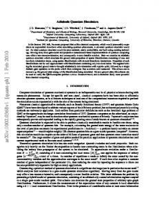
FIG. 2: Two isomorphic 4-vertex graphs G and G0 . 1.
Non-isomorphic graphs
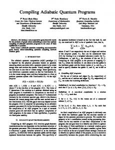
Here we use the GI AQA to examine a GI instance in which the two graphs G and G0 are non-isomorphic. The two graphs are shown in Figure 1. Each graph contains
0
3
}
}
}
}
1
0
2
3
} @ @
@
} @ @
@
@ @
@
}
@ @
@ @
@ @}
1
2
G0
G
FIG. 1: Two non-isomorphic 4-vertex graphs G and G0 .
4 vertices and 4 edges, however they are non-isomorphic. Examining Figure 1 we see that the degree sequence for G is {2, 2, 2, 2}, while that for G0 is {3, 2, 2, 1}. Since 1 these degree sequences areFigure different we know that G and G0 are non-isomorphic. Finally, the adjacency matrices A and A0 for G and G0 , respectively, are: 0 1 0 1 1 0 1 0 A= 0 1 0 1 1 0 1 0
0 0 0 0 A = 1 0 1 1
;
0
1 0 0 1
1 1 . 1 0
(16)
The GI AQA finds a non-zero final ground-state energy Egs = 4, and so correctly identifies these two graphs as non-isomorphic. It also finds that the final groundstate subspace has a degeneracy of 16. The linear maps associated with the 16 CBS that span this subspace give rise to the lowest cost linear maps of G relative to G0 . As these graphs are not isomorphic, these lowest cost maps have little inherent interest and so we do not list them.
2.
Isomorphic graphs
Here we examine the case of two isomorphic graphs G and G0 which are shown in Figure 2. Each graph contains 4 vertices and 5 edges, and both graphs have degree
sequence {3, 3, 2, 2}. By inspection of Figure 2, the associated adjacency matrices are, respectively, 0 1 1 1 0 1 1 1 Figure 2 1 0 0 1 1 0 1 0 . (17) ; A0 = A= 1 0 0 1 1 1 0 1 1 1 1 0 1 0 1 0 For these two graphs, the GI AQA finds a vanishing final ground-state energy Egs = 0 and so recognizes G and G0 as isomorphic. It also finds that the final ground-state subspace has a degeneracy of 4. The four CBS that span this subspace give four binary strings sb . These four binary strings in turn generate four integer strings s which are, respectively, the bottom row of four permutations (see Eq. (2)). Thus, not only does the GI AQA recognize G and G0 as isomorphic, but it also returns the 4 graph isomorphisms π1 , . . . , π4 that transform G → G0 while preserving adjacency: � � � � 0 1 2 3 0 1 2 3 π1 = ; π2 = ; 0 2 3 1 3 2 0 1 � � � � 0 1 2 3 0 1 2 3 π3 = ; π4 = . (18) 3 1 0 2 0 1 3 2 We will next explicitly show that π1 is a graph isomorphism; the reader can easily check that the remaining 3 permutations are also graph isomorphisms. The permutation matrix σ1 associated with π1 is 1 0 0 0 0 0 0 1 σ1 = . (19) 0 1 0 0 0 0 1 0 Under π1 , G is transformed to π1 (G) which is shown in Figure 3. It is clear from Figure 3 that vertices x and y are adjacent in G if and only if π1,x and π1,y are adjacent in π1 (G). The adjacency matrix for π1 (G) is σ1 Aσ1T which is easily shown to be 0 1 1 1 1 0 0 1 σ1 Aσ1T = . (20) 1 0 0 1 1 1 1 0 This agrees with the adjacency shown in π1 (G) in Figure 3. Comparison with Eq. (17) shows that σ1 Aσ1T = A0 .
7
0
3
} @ @ @
} @
@ @
@ @
@
1
0
} @ @
@
−→ @ @
}
@
@ @ @}
2
1
} @ @
2
}
4 @
@ @
}
}
@
@ @
@ @
@ @}
3
FIG. 3: Transformation of G produced by the permutation π1 .
Thus the permutation π1 does map G into G0 and preserve adjacency and so establishes that G and G0 are isomorphic. Figure 3 Finally, note that G and G0 are connected by exactly 4 graph isomorphisms. Examination of Figure 2 shows that the degree-3 vertices in G are vertices 0 and 2, while in G0 they are vertices 0 and 3. Since the degree of a vertex is preserved by a graph isomorphism [16], vertex 0 in G must be mapped to vertex 0 or 3 in G0 . Then vertex 2 (in G) must be mapped to vertex 3 or 0 (in G0 ), respectively. This then forces vertex 1 to map to vertex 1 or 2, and vertex 3 to map to vertex 2 or 1, respectively. Thus only 4 graph isomorphism are possible and these are exactly the 4 graph isomorphisms found by the GI AQA which appear in Eq. (18).
Non-isomorphic graphs
In this subsection we present GI instances involving pairs of non-isomorphic graphs. In Section IV B 1 we examine two instances of isospectral graphs; and in Section IV B 2 we look at three instances of strongly regular graphs. We shall see that the GI AQA correctly distinguishes all graph pairs as non-isomorphic.
3
}
}
2
N = 5 : It is known that no pair of graphs with less than 5 vertices is iso-spectral [28]. Figure 4 shows a pair of graphs G and G0 with 5 vertices which are isospectral and yet are non-isomorphic. Although both have 5 vertices and 4 edges, the degree sequence of G is {2, 2, 2, 2, 0}, while that of G0 is {4, 1, 1, 1, 1}. Since they
3
2
1
G0
FIG. 4: Two non-isomorphic 5-vertex iso-spectral graphs G and G0 .
have different degree sequences, it follows that G and G0 are non-isomorphic. TheFigure adjacency matrices A and A0 4 0 for G and G , respectively, are:
A=
0 1 0 1 0
1 0 1 0 0
0 1 0 1 0
1 0 1 0 0
0 1 0 0 1 0 0 ; A0 = 1 0 1 0 0 1 0 0
1 0 0 0 0
1 0 0 0 0
1 0 0 0 0
.
(21)
It is straight-forward to show that A and A0 have the same characteristic polynomial P (λ) = λ5 − 4λ3 and so G and G0 are iso-spectral. Numerical simulation of the dynamics of the GI AQA finds a non-zero final ground-state energy Egs = 5, and so the GI AQA correctly distinguishes G and G0 as non-isomorphic graphs. N = 6 : The pair of graphs G and G0 in Figure 5 are
} @ @ @
Iso-spectral graphs
The spectrum of a graph is the set containing all the eigenvalues of its adjacency matrix. Two graphs are iso-spectral if they have identical spectra. Nonisomorphic iso-spectral graphs are believed to be difficult to distinguish [8, 9]. Here we test the GI AQA on pairs of non-isomorphic iso-spectral graphs. The non-isomorphic pairs of iso-spectral graphs examined here appear in Ref. [28].
4
} ����DADA �� DA � � D A � � D A D A � � � � D A � � D A � � D A � � D A � � D A � � D A � � D A � � D A } � } � D} A}
G
0
1.
0
1
}
π1(G)
G
B.
0
1
2
4
} @
@ @
5
@ @} @ @ @
}
0 @ @
@
@ @}
3
}
G
}
1
} ��A � A A � A � A � A � AA} } � A �� A � A � A � A � A � AA� }
4
5
}
3
2 G0
FIG. 5: Two non-isomorphic 6-vertex iso-spectral graphs G and G0 .
iso-spectral and non-isomorphic. To see this, note that although both graphs have 6 vertices and 7 edges, the Figure 5 degree sequence of G is {5, 2, 2, 2, 2, 1}, while that of G0 is {3, 3, 3, 3, 1, 1}. Since their degree sequences are different, G and G0 are non-isomorphic. The adjacency matrices A
8 and A0 of G and G0 , respectively, are: 0 1 0 A= 0 0 1
1 0 0 0 0 1
0 0 0 0 0 1
0 0 0 0 1 1
0 0 0 1 0 1
0 1 1 1 0 1 1 0 1 ; A0 = 1 0 1 0 0 1 0 0 0
N = 4 : In Figure 6 we show two strongly regular 40 1 0 1 1 0
0 1 1 0 1 0
0 0 1 1 0 1
0 0 0 0 1 0
.
(22) Both A and A0 have the same characteristic polynomial P (λ) = λ6 − 7λ4 − 4λ3 + 7λ2 + 4λ − 1 which establishes that G and G0 are iso-spectral. Numerical simulation of the dynamics of the GI AQA finds a non-zero final ground-state energy Egs = 7, and so the GI AQA correctly distinguishes G and G0 as non-isomorphic graphs.
2.
Strongly regular graphs
As we saw in Section II A, the degree d(x) of a vertex x is equal to the number of vertices that are adjacent to x. A graph G is said to be k-regular if, for all vertices x, the degree d(x) = k. A graph is said to be regular if it is k-regular for some value of k. Finally, a strongly regular graph is a graph with ν vertices that is k-regular, and for which: (i) any two adjacent vertices have λ common neighbors; and (ii) any two non-adjacent vertices have µ common neighbors. The set of all strongly regular graphs is divided up into families, and each family is composed of strongly regular graphs having the same parameter values (ν, k, λ, µ). In this subsection we apply the GI AQA to pairs of non-isomorphic strongly regular graphs. An excellent test for this algorithm would be two non-isomorphic strongly regular graphs belonging to the same family as such graphs would then have the same order and degree sequence. Unfortunately, to find a family containing at least two non-isomorphic strongly regular graphs requires going to a family containing 16-vertex graphs. For example, the family (16, 9, 4, 6) contains two non-isomorphic strongly regular graphs. Since the GI AQA uses νdlog2 νe qubits, simulation of its quantum dynamics on 16-vertex graphs requires 64 qubits. This is hopelessly beyond the 20–22 qubit limit for such simulations discussed in the introduction to Section IV. As noted there, this hard limit restricts our simulations to graphs with no more than 7 vertices. Now the number of connected strongly regular graphs with ν = 4, 5, 6, 7 is 3, 2, 5, 1, respectively. For each of the values ν = 4, 5, 6, the strongly regular graphs are non-isomorphic as desired, however, each graph belongs to a different family. In light of the above remarks, the simulations reported in this subsection are restricted to pairs of connected non-isomorphic strongly regular graphs with ν = 4, 5, 6. Ideally we would have simulated the GI AQA on the above pair of 16-vertex strongly regular graphs, however the realities of simulating quantum systems on a classical computer made this test well beyond reach.
0
0
} @ @ @ @
3
} @ @ @
@
@ @
} @ @
@
@ @
1 @}
3
@ @}
} @ @
@
@ @
@
@
@ @
@
1
@ @}
@ @}
2
2
G0
G
FIG. 6: Two 4-vertex non-isomorphic strongly regular graphs G and G0 .
vertex graphs G and G0 . The parameters for G are ν = 4, k = 2, λ = 0, and µ = 2; while for G0 they are ν = 4, k = 3, λ = 2, and µ = 0.Figure It 6 is clear that G and G0 are non-isomorphic since they contain an unequal number of edges and different degree sequences. The adjacency matrices A and A0 for G and G0 are, respectively, 0 1 0 1 0 1 1 1 1 0 1 1 1 0 1 0 A= ; A0 = . (23) 0 1 0 1 1 1 0 1 1 0 1 0 1 1 1 0 Numerical simulation of the GI AQA dynamics finds a non-zero final ground-state energy Egs = 4 and so the GI AQA correctly distinguishes G and G0 as non-isomorphic. N = 5 : In Figure 7 we show two strongly regular 50
0
} @ @ @ @
4
3
}
}
@
@ @
@}
}
G
1
4
2
3
} @ @ ��A A � A@ � A @ A @ � @ � A @ A � } @} � A HH � A �� H� � H � H �� AA H � � HH � A � � H HH � �� A H A � �� HH H A} }� � �
1
2
G0
FIG. 7: Two 5-vertex non-isomorphic strongly regular graphs G and G0 .
vertex graphs G and G0 . The parameters for G are ν = 5, k = 2, λ = 0, and µ = 1; while for G0 they are ν = 5, k = 4, λ = 3, and µ = 0.Figure It 7 is clear that G and G0 are non-isomorphic since they contain an unequal number of edges and different degree sequences. The adjacency matrices A and A0 for G and G0 are, respectively, 0 1 0 0 1 0 1 1 1 1 1 0 1 0 0 1 0 1 1 1 A = 0 1 0 1 0 ; A0 = 1 1 0 1 1 . (24) 0 0 1 0 1 1 1 1 0 1 1 0 0 1 0 1 1 1 1 0
9 Numerical simulation of the GI AQA dynamics finds a non-zero final ground-state energy Egs = 10 and so the GI AQA correctly distinguishes G and G0 as non-isomorphic. N = 6 : In Figure 8 we show two strongly regular 6-
0 5
z @ @ @
z @ @
0
1
@
z @ @ @ @
@
@ @
@ @ @z
4
@
@ @z
@ @
z P PP Q AQ P A QQ PPP PP A Q PP Q PP A Qz A �hhhhhhPPP � hhhP A � hP hP hP hz z A� ( ((� Q (((�� � � QQ ((((((��� Q( z � �� � � � � �� � � ����� � � �� � �� � � �z
4
2
@ @z
1.
2
G0
G
FIG. 8: Two 6-vertex non-isomorphic strongly regular graphs G and G0 .
vertex graphs G and G0 . The parameters for G are ν = 6, k = 3, λ = 0, and µ = 3; while for G0 they are ν = 6, Figure 8 k = 4, λ = 2, and µ = 4. It is clear that G and G0 are non-isomorphic since they contain an unequal number of edges and different degree sequences. The adjacency matrices A and A0 for G and G0 are, respectively, 0 1 0 A= 1 0 1
1 0 1 0 1 0
0 1 0 1 0 1
1 0 1 0 1 0
0 1 0 1 0 1
0 1 1 1 0 0 1 1 1 ; A0 = 0 1 0 1 1 1 0 1 0
1 1 0 1 0 1
1 0 1 0 1 1
1 1 0 1 0 1
0 1 1 1 1 0
.
(25) Numerical simulation of the GI AQA dynamics finds a non-zero final ground-state energy Egs = 10 and so the GI AQA correctly distinguishes G and G0 as nonisomorphic.
C.
Cycle graphs
1
3
5
3
which are all the elements of Aut(G). By construction, the order of Aut(G) is equal to the degeneracy of the final ground-state subspace. In this subsection we apply the GI AQA to the: (i) cycle graphs C4 , . . . , C7 ; (ii) grid graph G2,3 ; and (iii) wheel graph W7 , and show that it correctly determines the automorphism group for all of these graphs.
Graph automorphisms
As noted in the Section IV introduction, we can find the automorphism group Aut(G) of a graph G using the GI AQA by considering a GI instance with G0 = G. To the best of our knowledge, such an application of a GI algorithm is new. Here the self-isomorphisms are permutations of the vertices of G that map G → G while preserving adjacency. Since G is always isomorphic to itself, the final ground-state energy will vanish: Egs = 0. The set of CBS |sb i that span the final ground-state subspace give rise to a set of binary strings sb that determine the integer strings s = s0 · · · sN −1 (see Section II B) that then determine the permutations π(s), � � 0 ··· i ··· N − 1 π(s) = , (26) s0 · · · si · · · sN −1
A walk W in a graph is an alternating sequence of vertices and edges x0 , e1 , x1 , e2 , · · · , el , xl , where the edge ei connects xi−1 and xi for 0 < i ≤ l. A walk W is denoted by the sequence of vertices it traverses W = x0 x1 · · · xl . Finally, a walk W = x0 x1 · · · xl is a cycle if l ≥ 3; x0 = xl ; and the vertices xi with 0 < i < l are distinct from each other and x0 . A cycle with n vertices is denoted Cn . The automorphism group of the cycle graph Cn is the dihedral group Dn [16]. The order of Dn is 2n, and it is generated by the two elements α and β that satisfy the following relations, αn = e;
β 2 = e;
αβ = βαn−1 ,
(27)
where e is the identity element. Because α and β are generators of Dn , each element g of Dn can be written as a product of appropriate powers of α and β: g = αi β j
(0 ≤ i ≤ n − 1 ; 0 ≤ j ≤ 1).
(28)
We now use the GI AQA to find the automorphism group of the cycle graphs Cn for 4 ≤ n ≤ 7. We will see that the GI AQA correctly determines Aut(Cn ) = Dn for these graphs. We will work out C4 in detail, and then give more abbreviated presentations for the remaining cycle graphs as their analysis is identical. N = 4: The cycle graph C4 appears in Figure 9. It
0
3
1
}
}
}
}
2
C4
FIG. 9: Cycle graph C4 .
contains 4 vertices and 4 edges; has degree sequence Figure 9
10 {2, 2, 2, 2}; and adjacency matrix 0 1 0 1 1 0 1 0 A= . 0 1 0 1 1 0 1 0
Under π∗ , C4 is transformed to π∗ (C4 ) which is shown in Figure 10. It is clear from Figure 10 that x and y are (29)
Numerical simulation of the GI AQA applied to the GI instance with G = C4 and G0 = G found a vanishing final ground-state energy Egs = 0. The GI AQA thus correctly identifies C4 as being isomorphic to itself. The simulation also found that the final ground-state subspace is 8-fold degenerate. Table I lists the integer strings TABLE I: Automorphism group Aut(C4 ) of the cycle graph C4 as found by the GI AQA. The first row lists the integer strings s = s0 s1 s2 s3 determined by the labels of the eight CBS |sb i that span the final ground-state subspace (see text). Each string s determines a graph automorphism π(s) via Eq. (26). The second row associates each integer string s in the first row with a graph automorphism π(s). It identifies the two strings that give rise to the graph automorphisms α and β that generate Aut(C4 ), and writes each graph automorphism π(s) as a product of an appropriate power of α and β. Note that e is the identity automorphism, and the product notation assumes the rightmost factor acts first. s = s0 s1 s2 s3 3012 2301 1230 0123 0321 3210 2103 1032 π(s) α α 2 α3 α4 = e β αβ α2 β α3 β
s = s0 s1 s2 s3 that result from the eight CBS |sb i that span the final ground-state subspace (see Sections II B and III). Each integer string s determines the bottom row of a permutation π(s) (see eq. (26)). We explicitly show that π(s), for the integer string s = 3210, is an automorphism of C4 . The reader can repeat this analysis to show that the seven remaining integer strings in Table I also give rise to automorphisms of C4 . Note that the CBS that span the final ground-state subspace determine all the graph automorphisms of C4 . This follows from the manner in which the GI AQA is constructed since each automorphism of C4 must give rise to a CBS with vanishing energy, and each CBS in the final ground-state subspace gives rise to an automorphism of C4 . These automorphisms form a group Aut(C4 ) and the GI AQA has found that the order of Aut(C4 ) is 8 which is the same as the order of the dihedral group D4 . The permutation π∗ ≡ π(s = 3210) is ! 0 1 2 3 π(3210) = , (30) 3 2 1 0 and the associated permutation matrix σ∗ ≡ σ(3210) is 0 0 0 1 0 0 1 0 σ(3210) = (31) . 0 1 0 0 1 0 0 0
0
1
}
3
}
2
}
}
}
}
−→
3
}
}
2
C4
0
1
π∗(C4)
FIG. 10: Transformation of C4 produced by the permutation π∗ .
adjacent in C4 if and only if π∗,x and π∗,y are adjacent in π∗ (C4 ). Thus π∗ is a permutation of the vertices of C4 Figure 10 that preserves adjacency and so is a graph automorphism of C4 . We can also show this by demonstrating that σ∗ Aσ∗T = A. Using Eqs. (29) and (31) it is easy to show that 0 1 0 1 1 0 1 0 (32) σ∗ Aσ∗T = . 0 1 0 1 1 0 1 0 This agrees with the adjacency of edges in π∗ (C4 ) appearing in Figure 10, and comparison with Eq. (29) shows that σ∗ Aσ∗T = A, confirming that π∗ is an automorphism of C4 . We now show that Aut(C4 ) is isomorphic to the dihedral group D4 by showing that the automorphisms π(3012) ≡ α and π(0321) ≡ β generate Aut(C4 ), and satisfy the generator relations (Eq. (27)) for D4 . The second row of Table I establishes that α and β are the generators of Aut(C4 ) as it shows that each element of Aut(C4 ) is a product of an appropriate power of α and β, and all possible products of powers of α and β appear in that row. Now notice that ! 0 1 2 3 α= (33) 3 0 1 2 corresponds to a clockwise rotation of C4 by 90◦ (see Figure 11) Thus four applications of α corresponds to a 360◦ rotation of C4 which leaves it invariant. Thus α4 = e. This can also be checked by composing α with itself four times using Eq. (33). This establishes the first of the generator relations in Eq. (27). Similarly, ! 0 1 2 3 β= (34) 0 3 2 1 corresponds to reflection of C4 about the diagonal passing through vertices 0 and 2 (see Figure 12). Thus two
11
0
1
}
3
}
0
}
0
}
} @ @ @ @
−→
3
}
}
2
4 }
2
1
C4
3
α(C4)
@
}
@ @
}
1
@}
}
2
C5
FIG. 11: Transformation of C4 produced by the automorphism α.
FIG. 13: Cycle graph C5 .
and adjacency matrix 0
1
}
}
Figure 11
0
3
}
}
0Figure 1 130 1 0 1 A=0 1 0 0 0 1 1 0 0
−→
3
}
}
2
C4
1
}
}
2
0 0 1 0 1
1 0 0 1 0
.
(37)
β(C4)
FIG. 12: Transformation of C4 produced by the automorphism β.
applications of β leaves C4 invariant, and so β 2 = e. This establishes the secondFigure of12the generator relations in Eq. (27). Finally, to show the third generator relation αβ = βα3 , we simply evaluate both sides of this relation and compare results. Using Table I we find that ! ! 0 1 2 3 0 1 2 3 αβ = 3 0 1 2 0 3 2 1 ! 0 1 2 3 = (35) 3 2 1 0 ! ! 0 1 2 3 0 1 2 3 βα3 = 0 3 2 1 1 2 3 0 ! 0 1 2 3 = . (36) 3 2 1 0 It is clear that αβ does equal βα3 . Thus we have shown that α and β: (i) generate Aut(C4 ); and (ii) satisfy the generator relations (Eq. (27)) for the dihedral group D4 , and so generate a group isomorphic to D4 . In summary, we have shown that the GI AQA found all eight graph automorphisms of C4 , and that the group formed from these automorphisms is isomorphic to the dihedral group D4 which is the correct automorphism group for C4 . N = 5: The cycle graph C5 appears in Figure 13. It has 5 vertices and 5 edges; degree sequence {2, 2, 2, 2, 2};
Numerical simulation of the GI AQA applied to the GI instance with G = C5 and G0 = G found a vanishing final ground-state energy Egs = 0. The GI AQA thus correctly identifies C5 as being isomorphic to itself. The simulation also found that the final groundstate subspace is 10-fold degenerate. Table II lists the TABLE II: Automorphism group Aut(C5 ) of the cycle graph C5 as found by the GI AQA. The odd rows list the integer strings s = s0 · · · s4 determined by the labels of the ten CBS |sb i that span the final ground-state subspace (see text). Each string s determines a graph automorphism π(s) via Eq. (26). Each even row associates each integer string s in the odd row preceding it with a graph automorphism π(s). It identifies the two strings that give rise to the graph automorphisms α and β that generate Aut(C5 ), and writes each graph automorphism π(s) as a product of an appropriate power of α and β. Note that e is the identity automorphism, and the product notation assumes the rightmost factor acts first. s = s0 · · · s4 π(s) s = s0 · · · s4 π(s)
40123 α 04321 β
34012 α2 10432 αβ
23401 α3 21043 α2 β
12340 α4 32104 α3 β
01234 α5 = e 43210 α4 β
integer strings s = s0 · · · s4 that result from the ten CBS |sb i that span the final ground-state subspace (see Sections II B and III). Each integer string s fixes the bottom row of a permutation π(s) (see eq. (26)) which is a graph automorphism of C5 . The demonstration of this is identical to the demonstration given for C4 and so will not be repeated here. Just as for Aut(C4 ), the graph automorphisms in Table II are all the elements of Aut(C5 ) which
12 is seen to have order 10. Note that this is the same as the order of the dihedral group D5 . We now show that Aut(C5 ) is isomorphic to the dihedral group D5 by showing that the graph automorphisms α = π(40123) and β = π(04321) generate Aut(C5 ), and satisfy the generator relations (Eq. (27)) for D5 . The second row of Table II establishes that α and β are the generators of Aut(C5 ) as it shows that each element of Aut(C5 ) is a product of an appropriate power of α and β, and that all possible products of powers of α and β appear in that row. Following the discussion for C4 , it is a simple matter to show that α corresponds to a 72◦ clockwise rotation of C5 . Thus 5 applications of α rotates C5 by 360◦ which leaves it invariant. Thus α5 = e which is the first of the generator relations in Eq. (27). Similarly, β can be shown to correspond to a reflection of C5 about a vertical axis passing through vertex 0 in Figure 13. Thus two applications of β leave C5 invariant. Thus β 2 = e which is the second generator relation in Eq. (27). Finally, using Table II, direct calculation as in Eqs. (35) and (36) shows that αβ = βα4 which establishes the final generator relation in Eq. (27). We see that α and β generate Aut(C5 ) and satisfy the generator relations for D5 and so generate a 10 element group isomorphic to D5 . In summary, we have shown that the GI AQA found all ten graph automorphisms of C5 , and that the group formed from these automorphisms is isomorphic to the dihedral group D5 which is the correct automorphism group for C5 . N = 6: The cycle graph C6 appears in Figure 14. It has 6 vertices and 6 edges; degree sequence
0 5
} @ @ @
@
@ @
1
}
} @ @ @ @
@ @}
@
@ @
2
@}
}
4
3
C6
FIG. 14: Cycle graph C6 .
{2, 2, 2, 2, 2, 2}; and adjacency 0 1 0 1 Figure 0 114 0 1 0 A= 0 0 1 0 0 0 1 0 0
matrix 0 0 1 0 1 0
0 0 0 1 0 1
1 0 0 0 1 0
.
(38)
Numerical simulation of the GI AQA applied to the GI instance with G = C6 and G0 = G found a vanishing final ground-state energy Egs = 0. The GI AQA
thus correctly identifies C6 as being isomorphic to itself. The simulation also found that the final groundstate subspace is 12-fold degenerate. Table III lists the
TABLE III: Automorphism group Aut(C6 ) of the cycle graph C6 as found by the GI AQA. The first and third rows list the integer strings s = s0 · · · s5 determined by the labels of the twelve CBS |sb i that span the final ground-state subspace (see text). Each string s determines a graph automorphism π(s) via Eq. (26). The second and fourth rows associate each integer string s in the first and third rows with a graph automorphism π(s). They also identify the two strings that give rise to the graph automorphisms α and β that generate Aut(C6 ), and write each graph automorphism π(s) as a product of an appropriate power of α and β. Note that e is the identity automorphism, and the product notation assumes the rightmost factor acts first. s = s0 · · · s5 501234 450123 345012 234501 123450 012345 π(s) α α2 α3 α4 α5 α6 = e s = s0 · · · s5 105432 210543 321054 432105 543210 054321 π(s) β αβ α2 β α3 β α4 β α5 β
integer strings s = s0 · · · s5 that result from the twelve CBS |sb i that span the final ground-state subspace (see Sections II B and III). Each integer string s fixes the bottom row of a permutation π(s) (see eq. (26)) which is a graph automorphism of C6 . The demonstration of this is identical to the demonstration given for C4 and so will not be repeated here. Just as for Aut(C4 ), the graph automorphisms in Table III are all the elements of Aut(C6 ) which is seen to have order 12. Note that this is the same as the order of the dihedral group D6 . We now show that Aut(C6 ) is isomorphic to the dihedral group D6 by showing that the graph automorphisms α = π(501234) and β = π(105432) generate Aut(C6 ), and satisfy the generator relations (Eq. (27)) for D6 . The second and fourth rows of Table III establish that α and β are the generators of Aut(C6 ) as they show that each element of Aut(C6 ) is a product of an appropriate power of α and β, and that all possible products of powers of α and β appear in these two rows. Following the discussion for C4 , it is a simple matter to show that α corresponds to a 60◦ clockwise rotation of C6 . Thus 6 applications of α rotates C6 by 360◦ which leaves it invariant. Thus α6 = e which is the first of the generator relations in Eq. (27). Similarly, β can be shown to correspond to a reflection of C6 about a vertical axis that bisects C6 . Thus two applications of β leave C6 invariant. Thus β 2 = e which is the second generator relation in Eq. (27). Finally, using Table III, direct calculation as in Eqs. (35) and (36) shows that αβ = βα5 which establishes the final generator relation in Eq. (27). We see that α and β generate Aut(C6 ) and satisfy the generator relations for D6 and so generate a 12 element group isomorphic to D6 . In summary, we have shown that the GI AQA found all twelve graph
13 automorphisms of C6 , and that the group formed from these automorphisms is isomorphic to the dihedral group D6 which is the correct automorphism group for C6 . N = 7: The cycle graph C7 appears in Figure 15. It has 7 vertices and 7 edges; degree sequence 0
} @ @ @ @
@
@ @
6
}
1
5
}
}
4
}
}
@}
2
s = s0 · · · s6 π(s) s = s0 · · · s6 π(s) s = s0 · · · s6 π(s) s = s0 · · · s6 π(s)
3
C7
FIG. 15: Cycle graph C7 .
{2, 2, 2, 2, 2, 2, 2}; and adjacency matrix 0 1 0 0 0 0 1 Figure 15 1 0 1 0 0 0 0 0 1 0 1 0 0 0 A= 0 0 1 0 1 0 0 . 0 0 0 1 0 1 0 0 0 0 0 1 0 1 1 0 0 0 0 1 0
TABLE IV: Automorphism group Aut(C7 ) of the cycle graph C7 as found by the GI AQA. The odd rows list the integer strings s = s0 · · · s6 determined by the labels of the fourteen CBS |sb i that span the final ground-state subspace (see text). Each string s determines a graph automorphism π(s) via Eq. (26). Each even row associates each integer string s in the odd row preceding it with a graph automorphism π(s). They also identify the two strings that give rise to the graph automorphisms α and β that generate Aut(C7 ), and write each graph automorphism π(s) as a product of an appropriate power of α and β. Note that e is the identity automorphism, and the product notation assumes the rightmost factor acts first.
(39)
Numerical simulation of the GI AQA applied to the GI instance with G = C7 and G0 = G found a vanishing final ground-state energy Egs = 0. The GI AQA thus correctly identifies C7 as being isomorphic to itself. The simulation also found that the final ground-state subspace is 14-fold degenerate. Table IV lists the integer strings s = s0 · · · s6 that result from the fourteen CBS |sb i that span the final ground-state subspace (see Sections II B and III). Each integer string s fixes the bottom row of a permutation π(s) (see eq. (26)) which is a graph automorphism of C7 . The demonstration of this is identical to the demonstration given for C4 and so will not be repeated here. Just as for Aut(C4 ), the graph automorphisms in Table IV are all the elements of Aut(C7 ) which is seen to have order 14. Note that this is the same as the order of the dihedral group D7 . We now show that Aut(C7 ) is isomorphic to the dihedral group D7 by showing that the graph automorphisms α = π(6012345) and β = π(0654321) generate Aut(C7 ), and satisfy the generator relations (Eq. (27)) for D7 . The second and fourth rows of Table IV establish that α and β are the generators of Aut(C7 ) as they show that each element of Aut(C7 ) is a product of an appropriate power of α and β, and that all possible products of powers of α and β appear in these two rows. Following the discussion for C4 , it is a simple matter to show that α corresponds to a 2π/7 radian clockwise rotation of
6012345 α 2345601 α5 0654321 β 4321065 α4 β
5601234 α2 1234560 α6 1065432 αβ 5432106 α5 β
4560123 α3 0123456 α7 = e 2106543 α2 β 6543210 α6 β
3456012 α4
3210654 α3 β
C7 . Thus 7 applications of α rotates C7 by 360◦ which leaves it invariant. Thus α7 = e which is the first of the generator relations in Eq. (27). Similarly, β can be shown to correspond to a reflection of C7 about a vertical axis that passes through vertex 0 in Figure 15. Thus two applications of β leave C7 invariant. Thus β 2 = e which is the second generator relation in Eq. (27). Finally, using Table IV, direct calculation as in Eqs. (35) and (36) shows that αβ = βα6 which establishes the final generator relation in Eq. (27). We see that α and β generate Aut(C7 ) and satisfy the generator relations for D7 and so generate a 14 element group isomorphic to D7 . In summary, we have shown that the GI AQA found all fourteen graph automorphisms of C7 , and that the group formed from these automorphisms is isomorphic to the dihedral group D7 which is the correct automorphism group for C7 .
2.
Grid graph G2,3
The grid graph G2,3 appears in Figure 16. It has 6 vertices and 7 edges; degree sequence {3, 3, 2, 2, 2, 2}; and adjacency matrix
0 1 1 A= 0 0 0
1 0 0 1 0 0
1 0 0 1 1 0
0 1 1 0 0 1
0 0 1 0 0 1
0 0 0 1 1 0
.
(40)
14
4
}
}
5
2
}
}
0
}
}
3
1
G2,3
FIG. 16: Grid graph G2,3 .
G2,3 has two reflection symmetries. The first is reflection about the horizontal line passing through vertices 2 and Figure 16 3, and the second is reflection about a vertical line that bisects G2,3 . Let α and β denote the permutation of vertices that these reflections produce. It follows from their definition that α = π(452301) and β = π(103254). They are the generators of the automorphism group of G2,3 : Aut(G2,3 ) = hα, βi. As reflections, they satisfy α2 = β 2 = e. Applying these reflections successively gives αβ = π(543210) which is a fourth symmetry of G2,3 . Applying these reflections in the reverse order, it is easy to verify that αβ = βα. Thus Aut(G2,3 ) is a 4 element Abelian group generated by the reflections α and β. Let us now compare this with the results found by the GI AQA. Numerical simulation of the GI AQA applied to the GI instance with G = G2,3 and G0 = G found a vanishing final ground-state energy Egs = 0. The GI AQA thus correctly identifies G2,3 as being isomorphic to itself. The simulation also found that the final ground-state subspace is 4-fold degenerate. Table V lists TABLE V: Automorphism group Aut(G2,3 ) of the grid graph G2,3 as found by the GI AQA. The first row lists the integer strings s = s0 · · · s5 determined by the labels of the four CBS |sb i that span the final ground-state subspace (see text). Each string s determines a graph automorphism π(s) via Eq. (26). The second row associates each integer string s in the first row with a graph automorphism π(s). They also identify the two strings that give rise to the graph automorphisms α and β that generate Aut(G2,3 ), and write each graph automorphism π(s) as a product of an appropriate power of α and β. Note that e is the identity automorphism, and the product notation assumes the rightmost factor acts first. s = s0 · · · s5 π(s)
452301 α
103254 β
012345 α = β2 = e 2
543210 αβ
the integer strings s = s0 · · · s5 that result from the four CBS |sb i that span the final ground-state subspace (see Sections II B and III). Each integer string s fixes the bottom row of a permutation π(s) (see eq. (26)) which
is a graph automorphism of G2,3 . The demonstration of this is identical to the demonstration given for C4 and so will not be repeated here. Notice that the GI AQA found the graph automorphisms π(452301) and π(103254) which implement the reflection symmetries of G2,3 described above. As they implement reflections, it follows that α2 = β 2 = e. The GI AQA also found the graph automorphism π(543210) which is the composite symmetry αβ described above. Using Table V, direct calculation as in Eqs. (35) and (36) shows that αβ = βα. Thus the GI AQA correctly found the two generators α and β of Aut(G2,3 ); correctly determined all 4 elements of Aut(G2,3 ); and correctly determined that Aut(G2,3 ) is an Abelian group. In summary, the GI AQA correctly determined the automorphism group of G2,3 .
3.
Wheel graph W7
The wheel graph W7 appears in Figure 17. It has 7 0 5
} @ @ @
@
@ @
} @ @ @
1
@
} @ @ @ @ @ @
6
@} @ @
@ @
@ @}
4
@
@
@ @
2
@}
@ @ @}
3
W7
FIG. 17: Wheel graph W7 .
vertices and 12 edges; degree sequence {6, 3, 3, 3, 3, 3, 3}; and adjacency matrix 0 1Figure 0 170 0 1 1 1 0 1 0 0 0 1 0 1 0 1 0 0 1 (41) A= 0 0 1 0 1 0 1 . 0 0 0 1 0 1 1 1 0 0 0 1 0 1 1 1 1 1 1 1 0 The automorphism group Aut(W7 ) is isomorphic to the dihedral group D6 which, as we have seen, has 12 elements and is generated by two graph automorphisms α and β that satisfy the generator relations in Eq. (27) with n = 6 and respectively, rotate W7 clockwise about vertex 6 by 60◦ , and reflect W7 about a vertical axis through vertex 6. The graph automorphisms of W7 thus fix vertex 6. Let us now compare this with the results found by the GI AQA. Numerical simulation of the GI AQA applied to the GI instance with G = W7 and G0 = G found a vanish-
15 ing final ground-state energy Egs = 0. The GI AQA thus correctly identifies W7 as being isomorphic to itself. The simulation also found that the final groundstate subspace is 12-fold degenerate. Table VI lists the TABLE VI: Automorphism group Aut(W7 ) of the wheel graph W7 as found by the GI AQA. The odd rows list the integer strings s = s0 · · · s6 determined by the labels of the twelve CBS |sb i that span the final ground-state subspace (see text). Each string s determines a graph automorphism π(s) via Eq. (26). Each even row associates each integer string s in the odd row preceding it with a graph automorphism π(s). They also identify the two strings that give rise to the graph automorphisms α and β that generate Aut(W7 ), and write each graph automorphism π(s) as a product of an appropriate power of α and β. Note that e is the identity automorphism, and the product notation assumes the rightmost factor acts first.
which establishes the final generator relation in Eq. (27). We see that α and β generate Aut(W7 ) and satisfy the generator relations for D6 and so generate a 12 element group isomorphic to D6 . In summary, we have shown that the GI AQA found all twelve graph automorphisms of W7 , and that the group formed from these automorphisms is isomorphic to the dihedral group D6 which is the correct automorphism group for W7 . V.
EXPERIMENTAL IMPLEMENTATION
In this section we express the GI problem Hamiltonian HP in a form more suitable for experimental implementation. We saw in Section II C that the eigenvalues of HP are given by the cost function C(s) which is reproduced here for convenience: C(s) = C1 (s) + C2 (s) + C3 (s),
s = s0 · · · s6 π(s) s = s0 · · · s6 π(s) s = s0 · · · s6 π(s) s = s0 · · · s6 π(s)
5012346 α 2345016 α4 1054326 β 4321056 α3 β
4501236 α2 1234506 α5 2105436 αβ 5432106 α4 β
3450126 α3 0123456 α6 = e 3210546 α2 β 0543216 α5 β
integer strings s = s0 · · · s6 that result from the twelve CBS |sb i that span the final ground-state subspace (see Sections II B and III). Each integer string s fixes the bottom row of a permutation π(s) (see eq. (26)) which is a graph automorphism of W7 . The demonstration of this is identical to the demonstration given for C4 and so will not be repeated here. Just as for Aut(C4 ), the graph automorphisms in Table VI are all the elements of Aut(W7 ) which is seen to have order 12. Note that this is the same as the order of the dihedral group D6 . We now show that Aut(W7 ) is isomorphic to the dihedral group D6 by showing that the graph automorphisms α = π(5012346) and β = π(1054326) generate Aut(W7 ), and satisfy the generator relations (Eq. (27)) for D6 . The second and fourth rows of Table VI establish that α and β are the generators of Aut(W7 ) as they show that each element of Aut(W7 ) is a product of an appropriate power of α and β, and that all possible products of powers of α and β appear in these two rows. Following the discussion for C4 , it is a simple matter to show that α corresponds to a 60◦ clockwise rotation about vertex 6 of W7 . Thus 6 applications of α rotates W7 by 360◦ which leaves it invariant. Thus α6 = e which is the first of the generator relations in Eq. (27). Similarly, β can be shown to correspond to a reflection of W7 about a vertical axis passing through vertex 6 of W7 . Thus two applications of β leave W7 invariant. Thus β 2 = e which is the second generator relation in Eq. (27). Finally, using Table VI, direct calculation as in Eqs. (35) and (36) shows that αβ = βα5
(42)
with C1 (s) =
N −1 X M X
δsi ,α
(43)
i=0 α=N
C2 (s) =
N −2 N −1 X X
δsi ,sj ,
(44)
i=0 j=i+1
C3 (s) = kσ(s)Aσ T (s) − A0 ki .
(45)
Here s = s0 · · · sN −1 is the integer string derived from the binary string sb = (s0 · · · sU −1 ) · · · (s(N −1)U · · · sN U −1 ) via Eqs. (6) and (7) with U = dlog2 N e. The matrix σ(s) was defined in Eq. (8) as ( 0, if sj > N − 1 σi,j (s) = (46) δi,sj , if 0 ≤ sj ≤ N − 1. Note that σi,j (s) can be written more compactly as σi,j (s) = δi,sj
M Y α=N
� 1 − δsj ,α .
(47)
We see from Eqs. (42)–(45) and (47) that the sdependence of C(s) enters through the Kronecker deltas. This type of s-dependence is not well-suited for experimental implementation and so our task is to find a more convenient form for the Kronecker delta. We begin with δa,b in the case where a, b ∈ {0, 1}. Here we write ( 0 (a 6= b) 2 δa,b = (a + b − 1) = (48) 1 (a = b), which can be checked by inserting values for a and b. Now consider δs,k when s and k are U -bit integers. The
16 binary decompositions of s and k are s =
U −1 X
i
(49)
i
(50)
si (2)
i=0
k =
U −1 X
ki (2) .
i=0
For s and k to be equal, all their corresponding bits must be equal. Thus we can write δs,k =
U −1 Y
δsi ,ki
i=0
=
U −1 Y i=0
( 2
(si + ki − 1) =
1 0
(all si = ki ) (51) (some si 6= ki ).
Eq. (51) allows each Kronecker delta appearing in C(s) to be converted to a polynomial in the components of the integer string s. From Eqs. (43) and (44) we see that C1 (s) and C2 (s) are each 2U -local. For C3 (s) we must write σ(s)Aσ T (s) in a form that makes the Kronecker deltas explicit. Using Eq. (47), we have σ(s)Aσ T (s) =
N −1 X
σli (s)Aij σmj (s)
i,j=0
=
N −1 X
( δl,si
i,j=0
×
M Y α=N
δm,sj
T (LN ) = T1 (LN ) + T2 (LN ) + T3 (LN ) = O(L2N ). The initial Hamiltonian Hi contains one term for each qubit (see Eq. (15)) and so the number of terms in Hi is LN . Thus the total number of terms in the full time-dependent Hamiltonian H(t) is O(L2N ) and so scales quadratically with the number of qubits LN . Clearly, the degree of difficulty associated with experimentally implementing a quantum algorithm depends strongly on the architecture of the hardware on which it is to be run. The simplest situation would be an architecture which allows an arbitrary number of qubits to be simultaneously coupled, independently of where they were located on the processor. Unfortunately, such a hardware architecture does not presently exist. For hardware platforms designed to run adiabatic quantum optimization algorithms, the D-Wave hardware is furthest along [29]. Each qubit on the D-Wave processor couples to at most six neighboring qubits, and only two-qubit Ising coupling interactions are possible. The initial Hamiltonian Hi (see Eq. (15)) is easily programmed onto the hardware. However, a problem Hamiltonian HP which is not of Ising form is more challenging, requiring an embedding procedure that: (i) reduces all k-local interactions with k ≥ 3 to 2-local form; and (ii) two-qubit coupling interactions that match the hardware’s Chimera couplinggraph. A procedure for carrying out this reduction based on Ref. [15] is described in Appendix B. Alternative approaches appear in Refs. [30] and [31].
) (1 − δsi ,α ) Aij
M Y β=N
1 − δsj ,β
�
. (52)
Inserting Eq. (51) into Eq. (52), we see that σ(s)Aσ T (s)− A0 is 4U (M − N + 1)-local. If we use the L1 -norm (L2 norm) in Eq. (45), then we see that C3 (s) is 4U (M − N + 1)-local (8U (M − N + 1)-local). The number of terms in C(s), and thus in HP , follows straight-forwardly from Eqs. (43)-(45). Starting with C1 (s), there is a term for each value of i and α that appears in the sum. There are thus T1 = N (M − N + 1) terms in C1 (s). From Eq. (5), M = 2U − 1, where U = dlog2 N e and N is the number of vertices in each graph appearing in the GI instance. It follows from the definition of U that M < 2N and so T1 < N (N + 1). Recall from Section III that the number of qubits LN needed for an N -vertex GI instance is LN = N dlog2 N e. Thus T1 < (LN /dlog2 N e)(LN /dlog2 N e + 1) < CL2N , where C is an appropriate constant. Thus T1 (LN ) = O(L2N ). A similar analysis shows that the number of terms in C2 (s) is T2 (LN ) = O(L2N ). Finally, C3 (s) is the Li -norm of an N × N matrix. For the L1 -norm used in our simulations, the number of terms in C3 (s) is T3 = N 2 . Following the above analysis, this gives T3 (LN ) = O(L2N ). Putting everything together gives that the total number of terms associated with C(s), and so also HP , is
VI.
SUBGRAPH ISOMORPHISM PROBLEM
An instance of the SubGraph Isomorphism (SGI) problem consists of an N -vertex graph G and an n-vertex graph H with n ≤ N . The question to be answered is whether G contains an n-vertex subgraph that is isomorphic to H. The SGI problem is known to be NPComplete [32] and is believed to be more difficult to solve than the GI problem. Here we show how an instance of SGI can be converted into an instance of a COP whose cost function has a minimum value that vanishes when G contains a subgraph isomorphic to H, and is greater than zero otherwise. The SGI cost function will be seen to be a natural generalization of the GI cost function given in Eqs. (9)–(12). The SGI COP can then be solved using adiabatic quantum evolution as was done for the GI problem. As with the GI problem, we would like to determine whether there exists an isomorphism π of G that produces a new graph π(G) that contains H as a subgraph. Just as with the GI problem, we consider linear maps σ(s) (see Eqs. (6)–(8)) that transform the adjacency ma˜ trix A of G to A(s) = σ(s)Aσ T (s). We then search π(G) to determine whether there is a subset of n vertices that yields a subgraph that is equal to H. To begin the process of converting an SGI instance � into an instance of a COP, let: (i) α label all the N n ways of choosing n vertices from the N vertices in π(G); and
17 (ii) |ii (|αi i) be an n-component (N -component) vector whose i-th (αi -th) component is 1, and all other components are 0. Thus α labels the choice (α0 , . . . , αn−1 ) of n vertices out of the N vertices of π(G). We now show that an n × N matrix Pα can be used to form an n × n matrix Aα (s) whose matrix elements are the matrix elements of ˜ A(s) associated with the n vertices appearing in α. To that purpose, define Pα =
n−1 X i=0
|iihαi |,
(53)
T ˜ Aα (s) = Pα A(s)P α,
(54)
where
C(s) = C1 (s) + C2 (s) + C3 (s),
N −1 X
˜ A(s) =
A˜l,m (s)|lihm|.
(55)
l,m=0
It follows from these definitions that Aα (s) = =
n−1 X i,=0
|iihαi |
n−1 X
N −1 X
A˜l,m (s)|lihm|
n−1 X j=0
l,m=0
A˜αi ,αj (s)|iihj|.
|αj ihj| (56)
i,j=0
Thus the matrix elements (Aα )i,j (s) are precisely the matrix elements A˜αi ,αj (s) associated with all possible pairs of vertices drawn from (α0 , . . . , αn−1 ). The matrix Aα (s) is thus the adjacency matrix for the subgraph gα composed of the vertices appearing in α, along with all the edges in π(G) that join them. With Aα (s), we can, as in the GI problem, test whether gα is equal to H by checking whether ||Aα (s) − A0 ||i vanishes or not. Here A0 is the adjacency matrix of the graph H, and ||O||i is the Li -norm of O. We can now define a cost function whose minimum value vanishes if and only if G contains a subgraph g that is isomorphic to H. Because the transformation σ(s) must be a permutation matrix when g is isomorphic to H, we again introduce the penalty functions C1 (s) and C2 (s) used in the GI COP to penalize those integer strings s that produce a σ(s) that is not a permutation matrix: C1 (s) =
N −1 X M X
δsi ,α
(57)
i=0 α=N
C2 (s) =
N −2 N −1 X X
δsi ,sj .
(58)
i=0 j=i+1
The final penalty function C3 (s) for the SGI problem generalizes the one used in the GI problem. It is defined to be C3 (s) =
N (Y n)
α=1
� where the product is over all N ways of choosing n n vertices out of N vertices. Note that C3 (s) vanishes if and only if G contains an n-vertex subgraph isomorphic to H. This follows since, if G contains an n-vertex subgraph g isomorphic to H, there exists a permutation π(s) of G that has an n-vertex subgraph that is equal to H. Thus, for this s, there is a choice α of n vertices that gives a subgraph for which Aα (s) − A0 = 0. It follows from Eq. (59) that C3 (s) = 0. On the other hand, if C3 (s) = 0, it follows that at least one of the factor on the RHS of Eq. (59) vanishes. Thus there is a choice α of n vertices for which ||Aα (s) − A0 ||i = 0. Thus Aα (s) = A0 , and so G has a subgraph isomorphic to H. The cost function for the SGI problem is now defined to be
||Aα (s) − A0 ||i ,
(59)
(60)
where C1 (s), C2 (s), and C3 (s) are defined in Eqs. (57)– (59). This gives rise to the following COP: SubGraph Isomorphism COP: Given an N -vertex graph G and an n-vertex graph H with n ≤ N , and the associated cost function C(s) defined in Eq. (60), find an integer string s∗ that minimizes C(s). By construction: (i) C(s∗ ) = 0 if and only if G contains a subgraph isomorphic to H, and σ(s∗ ) is the permutation matrix that transforms G into a graph π(G) that has H as a subgraph; and (ii) C(s∗ ) > 0 otherwise. As with the GI COP, the SGI COP can be solved using adiabatic quantum evolution. The quantum algorithm for SGI begins by preparing the L = N dlog2 N e qubit register in the ground-state of Hi (see Eq. (15)) and then driving the qubit register dynamics using the timedependent Hamiltonian H(t) = (1 − t/T )Hi + (t/T )HP . Here the problem Hamiltonian HP is defined to be diagonal in the computational basis |sb i and to have associated eigenvalues C(s), where s is found from sb according to Eqs. (6)–(7). At the end of the evolution the qubits are measured in the computational basis. The outcome is the bit string s∗b so that the final state of the register is |s∗b i and its energy is C(s∗ ), where s∗ is the integer string derived from s∗b . In the adiabatic limit, C(s∗ ) will be the ground-state energy, and if C(s∗ ) = 0 ( > 0) the algorithm concludes that G contains (does not contain) a subgraph isomorphic to H. In the case where G does contain a subgraph isomorphic to H, the algorithm also returns the permutation π∗ = π(s∗ ) that converts G to the graph π∗ (G) that contains H as a subgraph. Note that any real application of AQO will only be approximately adiabatic. Thus the probability that the final energy C(s∗ ) will be the ground-state energy will be 1 − �. In this case the SGI quantum algorithm must be run k ∼ O(ln(1 − δ)/ ln �) times so that, with probability δ > 1 − �, at least one of the measurements will return the ground-state energy. We can make δ arbitrarily close to 1 by choosing k sufficiently large.
18 VII.
1.
SUMMARY
In this paper we have presented a quantum algorithm that solves arbitrary instances of the Graph Isomorphism problem and which provides a novel approach for finding the automorphism group of a graph. We numerically simulated the algorithm’s quantum dynamics and showed that it correctly: (i) distinguished nonisomorphic graphs; (ii) recognized isomorphic graphs; and (iii) determined the automorphism group of a given graph. We also discussed the quantum algorithm’s experimental implementation, and showed how it can be generalized to give a quantum algorithm that solves arbitrary instances of the NP-Complete SubGraph Isomorphism problem. As explained in Appendix A, the minimum energy gap for an adiabatic quantum algorithm largely determines the algorithm’s computational complexity. Determining this gap in the limit of large problem size is currently an important open problem in adiabatic quantum computing (see Section IV). It is thus not possible to determine the computational complexity of adiabatic quantum algorithms in general, nor, consequently, of the specific adiabatic quantum algorithms presented in this paper. Adiabatic quantum computing has been shown to be equivalent to the circuit-model of quantum computing [12–14], and so development of adiabatic quantum algorithms continues to be of great interest.
Acknowledgments
We thank W. G. Macready and D. Dahl for many interesting discussions, and F. G. thanks T. Howell III for continued support.
Quantum adiabatic theorem
Consider a quantum system coupled to an environment that changes slowly over a time T . The dynamical evolution of its state |ψ(t)i is determined by the Schrodinger equation, which will be driven by a slowly-varying Hamiltonian H(t). The system’s Hilbert space is assumed to be finite-dimensional with dimension d. Thus at each instant t there will be d instantaneous energy eigenstates |Ek (t)i satisfying H(t)|Ek (t)i = Ek (t)|Ek (t)i,
with E0 (t) ≤ E1 (t) ≤ · · · ≤ Ed−1 (t). Now suppose that we initially prepare the quantum system in the instantaneous energy eigenstate |Ek (0)i of the initial Hamiltonian H(0). The quantum adiabatic theorem states that, in the limit T → ∞, the final state |ψ(T )i will be (to within a phase factor) the instantaneous energy eigenstate |Ek (T )i of the final Hamiltonian H(T ). Note that in our discussions of adiabatic quantum computing, the initial state will always be the ground state of H(0): |ψ(0)i = |E0 (0)i. For reasons that will become clear below, the energy gap, ∆(t) = E1 (t) − E0 (t), separating the two lowest instantaneous energy-levels proves to be extremely important in adiabatic quantum computing. Although it is possible to prove the quantum adiabatic theorem for systems with a vanishing energy gap [41], the rate of convergence to the adiabatic limit can be arbitrarily slow. On the other hand, when the gap ∆(t) is non-vanishing for 0 ≤ t ≤ T , it is possible to estimate how large T must be for the dynamics to be effectively adiabatic. Starting from the observation that for adiabatic dynamics there will be negligible probability to find the quantum system at t = T in an energy-level other than the ground state, a straightforward analysis [19, 20] leads to the following adiabaticity constraint:
APPENDIX A: QUANTUM ADIABATIC THEOREM
The question of how the state of a physical system changes when the system’s environment undergoes a slow variation is an old one. For quantum systems, the answer is contained in the quantum adiabatic theorem which was proved by Born and Fock not long after the birth of quantum mechanics [33]. Subsequent work relaxed a number of the assumptions underlying the original proof [34–43], thereby widening the theorem’s range of validity. As the physical setting for the quantum adiabatic theorem occurs often, it forms the foundation for many important applications in atomic, molecular, and chemical physics. Recently, it has been used as the basis for a novel alternative approach to quantum computing known as adiabatic quantum computing [21, 22]. In this Appendix we provide a brief review of the quantum adiabatic theorem (Appendix A 1) and then describe how it is used in adiabatic quantum computing (Appendix A 2).
(A1)
T �
~M , ∆2
(A2)
where ˜ dH(s) M = max hE1 (s)| |E0 (s)i , 0≤s≤1 ds
(A3)
∆ = min [E1 (s) − E0 (s)] ,
(A4)
0≤s≤1
˜ s = t/T , and H(s) = H(sT ). The quantity ∆ is the minimum energy gap arising during the adiabatic evolution. The quantum adiabatic theorem provides a mechanism for traversing a path |ψ(t)i through Hilbert space that begins at a given state |ψi i and ends at a desired final state |ψf i. To see this, let Hi and Hf be local Hermitian operators whose ground states are |ψi i and |ψf i, respectively. An Hermitian operator is local if it couples at most k particles, with k finite. Suppose that we can apply a time-dependent Hamiltonian H(t) over a timeinterval 0 ≤ t ≤ T , with H(0) = Hi , and H(T ) = Hf .
19 Suppose further that we prepare our quantum system in the ground state |ψi i of Hi , and then apply H(t) to it. In the limit T → ∞, the quantum adiabatic theorem guarantees that the system at time T will be in the desired state |ψf i. The outcome is thus a continuous path from |ψi i to |ψf i. 2.
Adiabatic quantum computing
To connect this discussion to quantum computing, imagine that there is a computational problem we would like to solve, and that we are able to construct a local Hamiltonian Hf whose ground state |ψf i encodes the solution to our problem. Often, the computational basis states can be chosen to be the eigenstates of HP . Our GI problem Hamiltonian HP is an example of such a Hamiltonian (see Section III). Let Hi be a local Hamiltonian operator whose ground state |ψi i is easy to prepare (e. g. see Eq. (15)). In adiabatic quantum computing, the procedure presented in the preceding paragraph is applied with |ψ(0)i = |ψi i and H(t) tracing out a path from Hi to Hf (in the space of Hermitian operators). Originally, Ref. [21] chose H(t) to linearly interpolate from Hi to Hf : H(t) = (1 − t/T ) Hi + (t/T ) Hf .
(A5)
˜ Writing s = t/T and H(s) = H(sT ) gives ˜ H(s) = (1 − s) Hi + sHf .
(A6)
More general interpolation schemes are possible: H(t) = A(t)Hi + B(t)Hf , where we require A(0) = 1 (B(0) = 0) and A(T ) = 0 (B(T ) = 1). See, for example, Refs. [15, 25, 27]. By choosing T sufficiently large, the final state |ψ(T )i can be brought arbitrarily close to |ψf i. An appropriate measurement then yields |ψf i with probability close to 1, and thus yields the desired solution to our computational problem. Adiabatic quantum computing thus finds the solution to a computational problem by homing in on the ground state |ψf i of Hf which encodes the solution. The homing mechanism is provided by the quantum adiabatic theorem. It has been shown that adiabatic quantum computing has the same computational power as the circuit model for quantum computing [12–14]. It thus provides an important alternative approach to quantum computing that is especially well suited to problems that reduce to quantum state generation. We are now in a position to state the protocol for the adiabatic quantum evolution (AQE) algorithm [21]: 1. Prepare an n-qubit quantum register in the ground state |ψi i of Hi . 2. At t = 0, apply H(t) to the quantum register for a time T . 3. At time t = T , measure the qubits in the computational basis.
Because the computational basis states are typically the eigenstates of Hf , the final measurement leaves the qubits in an eigenstate of Hf . In the adiabatic limit T → ∞, the final measurement leaves the qubits in the ground-state of Hf (which encodes the solution we are trying to find) with probability Psuccess → 1. Now for large, but finite T , the Schrodinger dynamics is approximately adiabatic. Thus, with probability 1 − �, the measurement returns the problem solution. In this case the AQE algorithm must be run more than once. Suppose we run it κ times. The probability that we do not get the problem solution in any of the κ runs is �κ . We can make this probability take an arbitrarily small value �˜ by choosing κ ∼ O(log(1/˜ �)). Thus with probability arbitrarily close to 1, one of the κ measurement results will yield the problem solution. The adiabaticity constraint (see Eq. (A2)) specifies a lower bound which the runtime T must exceed if the Schrodinger dynamics is to be effectively adiabatic. In all applications of interest to date, the matrix element M appearing in this constraint scales polynomially with problem size N . So long as this is true, Eq. (A2) indicates that the scaling behavior of the runtime T (N ) is determined by the scaling behavior of the minimum gap ∆(N ). Now, if at t = 0 the quantum register is prepared in the ground state of the initial Hamiltonian H(0), and its dynamics is effectively adiabatic, its state at later times will be effectively restricted to the subspace spanned by the instantaneous ground and first excited states. Standard arguments [44] indicate that, in the absence of symmetry, these two energy-levels will typically not cross. Thus the minimum gap ∆(N ) will typically not vanish, and Eq. (A2) indicates that an effectively adiabatic dynamics can be obtained with finite T (N ). An algorithm, classical or quantum, is said to efficiently (inefficiently) solve a computational problem if its runtime scales polynomially (super-polynomially) with problem size. Thus, if ∆(N ) scales inverse polynomially (super-polynomially) with N , then T (N ) will scale polynomially (super-polynomially) with N , and the AQE algorithm will be an efficient (inefficient) algorithm. We see that the scaling behavior of the minimum gap ∆(N ) largely controls the computational complexity of the AQE algorithm.
APPENDIX B: EMBEDDING PROCEDURE FOR D-WAVE HARDWARE
This Appendix briefly describes the embedding procedure used in Ref. [15] to program a non-Ising problem Hamiltonian HP onto a D-Wave One processor. The processor architecture is shown in Fig. 18. This procedure also applies to a D-Wave Two processor. As discussed in Section III, the GI algorithm presented in this paper constructs HP to: (i) be diagonal in the computational basis {|a0 · · · aL−1 i : ai = 0, 1}; and
20 correspond to available couplings on the processor (see Fig. 18). Procedures for removing each of these obstacles are presented, respectively, in Appendices B 1 and B 2. We summarize these procedures in Appendix B 3. To keep the discussion concrete, we examine a single k-qubit coupling term A = a1 · · · ak with ai = 0, 1. The resulting procedure must then be applied to each term in C(a).
1
5
9
13
17
21
25
29
2
6
10
14
18
22
26
30
3
7
11
15
19
23
27
31
4
8
12
16
20
24
28
32
33
37
41
45
49
53
57
61
34
38
42
46
50
54
58
62
35
39
43
47
51
55
59
63
36
40
44
48
52
56
60
64
65
69
73
77
81
85
89
93
66
70
74
78
82
86
90
94
67
71
75
79
83
87
91
95
68
72
76
80
84
88
92
96
97
101
105
109
113
117
121
125
P (a1 , a2 ; b) = a1 a2 − 2(a1 + a2 )b + 3b.
98
102
106
110
114
118
122
126
Notice that P (a1 , a2 ; b) = 0 (> 0) when the input values for a1 , a2 , and b satisfy b = a1 a2 (b 6= a1 a2 ). Now consider the quadratic cost function
99
103
107
111
115
119
123
127
100
104
108
112
116
120
124
128
1.
Reduction to pairwise coupling
Here we describe how to reduce a k-qubit coupling term A = a1 · · · ak with ai = 0, 1 to a sum of 2-qubit (viz. pairwise) coupling terms. We first show how to reduce a 3-qubit coupling term to pairwise coupling terms (Appendix B 1 a), and then use lessons learned to reduce the k-qubit term A to pairwise coupling (Appendix B 1 b). a.
3-qubit case
We begin by showing how to reduce a 3-qubit coupling term a1 a2 a3 to pairwise coupling by introducing: (i) an ancillary variable b which takes only two values {0, 1}; and (ii) the penalty function (B1)
h(b) = ba3 + µP (a1 , a2 ; b)
FIG. 18: Layout of qubits and couplers for a D-Wave One processor. The processor architecture is a 4 × 4 array of unit cells, with each unit cell containing 8 qubits. Within a unit cell, each of the 4 qubits in the left-hand partition (LHP) connects to all 4 qubits in the right-hand partition (RHP), and vice versa. A qubit in the LHP (RHP) of a unit cell also connects to the corresponding qubit in the LHP (RHP) in the units cells above and below (to the left and right of) it. Most qubits couple to 6 neighbors. Qubits are labeled from 1 to 128, and edges between qubits indicate couplers which may take programmable values. Grey qubits indicate usable qubits, while white qubits indicate qubits which, due to fabrication defects, could not be calibrated to operating tolerances and were not used.
(ii) have eigenvalues C(a), where a = a0 · · · aL−1 , L is the number of qubits, and C(a) is given by Eqs. (42)-(45) with s → a. The cost function C(a) is not yet ready for experimental implementation for two reasons. First, there are k-qubit interactions with k > 2 which cannot be implemented as the processor can only couple pairs of qubits; and second, two-qubit couplings may not
for given values of µ, a1 , and a2 . For µ sufficiently large, h(b) is minimized when the value of b satisfies the equality constraint b∗ = a1 a2 . As noted above, for this optimal value of b, the penalty function P (a1 , a2 ; b∗ ) = 0, and so the optimum cost h(b∗ ) is h(b∗ ) = b∗ a3 + P (a1 , a2 ; b∗ ) = a1 a2 a3 , where b∗ = a1 a2 has been used in going from the first to the second line. Thus, for values of b satisfying the equality constraint b = a1 a2 , the cost function h(b), which is a sum of 2-qubit coupling terms, reproduces the 3-qubit coupling term a1 a2 a3 . By choosing µ sufficiently large, values of b that do not satisfy the equality constraint can be pushed to large cost (viz. energy), making such b values inaccessible during adiabatic quantum evolution. b.
k-qubit case
To reduce the k-qubit coupling term A = a1 · · · ak to pairwise coupling we: (i) introduce ancillary bit variables b2 , · · · , bk−1 ; and (ii) impose the constraints bk−1 =
21 ak−1 ak and bj = aj bj+1 (j = 2, · · · , k − 2) through the penalty function P (a; b) = P (ak−1 , ak ; bk−1 ) +
k−2 X
P (aj , bj+1 ; bj ),
j=2
where a = (a1 , · · · , ak ), b = (b2 , · · · , bk−1 ) and P (a, b; c) is defined in Eq. (B1). The quadratic cost function CA (a, b) is defined to be CA (a, b) = a1 b2 + µ P (a; b). We require that the optimal values (a∗ , b∗ ) satisfy the k − 1 imposed constraints so that P (a∗ , b∗ ) = 0. For optimal values, the cost function evaluates to CA (a∗ , b∗ ) = a∗1 b∗2 + µP (a∗ , b∗ ) = a∗1 a∗2 b∗3 . = .. = a∗1 · · · a∗k−2 b∗k−1 = a∗1 · a∗k , where (in the interests of clarity) we have introduced the constraints one at a time in going from one line to the next. Here µ is a penalty weight whose value is chosen large enough to freeze out non-optimal values of a and b during adiabatic quantum evolution. Thus, for values of a and b satisfying the k − 1 equality constraints, and for µ sufficiently large, the cost function CA (a, b), which is a sum of 2-qubit coupling terms, reproduces the k-qubit coupling term A = a1 · · · ak as desired.
still not be experimentally realizable on a D-Wave processor as the pairwise couplings arising in CA (a, b) may not match the two-qubit couplings available on the processor. The primal graph of a quadratic cost function such as CA (a, b) is the graph whose vertices are the qubit variables, and whose edges indicate pairwise-coupled qubits. An arbitrary primal graph can be embedded into a sufficiently large qubit graph having the structure of Fig. 18. An embedding maps a primal graph vertex to one or more vertices in the qubit graph, where the image vertices form a connected subgraph of the qubit graph. The string of connected qubits are linked together with strong ferromagnetic couplings so that in the lowest energy state, these qubits have identical Bloch vectors. For example, to couple qubits 104 and 75 in Fig. 18 (which are not directly coupled) with coupling strength J , we ferromagnetically couple qubits 104, 112, and 107 using strongly negative J104,112 and J107,112 values. Qubits 107 and 75 are directly coupled by the processor and so the desired coupling J is applied to the edge (viz. coupler J107,75 ) connecting qubits 107 and 75: J107,75 = J . The ferromagnetic chain thus effects the desired coupling of qubits 104 and 75. This embedding procedure must be carried out for each pair of primal graph vertices joined by an edge whose associated qubits are not directly coupled in the processor architecture.
3.
Summary
A cost function with only pairwise coupling such as results from the procedure described in Appendix B 1 may
By combining the procedures described in this Appendix it is possible to transform any cost function C(a) into a quadratic cost function with pairwise couplings that matches the couplings specified by the processor architecture. The trade-off is the introduction of ancilla qubits that are needed to reduce the coupling interactions to pairwise coupling and to match the 2-qubit couplings available on the processor.
[1] J. K¨ obler, U. Sch¨ oning, and J. Tor´ an, The Graph Isomorphism Problem (Birkh¨ auser, Boston, 1993). [2] S. Arora and B. Barak, Computational Complexity (Cambridge University Press, New York, 2009). [3] R. Jozsa, Computing in Science and Engineering, 3, 34 (2001). [4] E. Bernstein and U. Vazarani, in Proc. 25th Annual ACM Symposium on the Theory of Computing, edited by R. Kosaraju, D. Johnson, and A. Aggarwal (ACM, San Diego, 1993), p. 11. [5] C. Moore, A. Russell, and L. J. Schulman, in 46th Annual IEEE Symposium on Foundations of Computer Science, edited by E. Tardos (IEEE, Los Alamitos, CA, 2005), p. 479. [6] V. Gudkov and S. Nussinov, arXiv.org:condmat/0209112v2 (2002).
[7] T. Rudolph, arXiv.org:quant-ph/0206068v1 (2002). [8] S. Shiau, R. Joynt, and S.N. Coppersmith, Quantum Inf. Compt. 5, 492 (2005). [9] J. K. Gamble, M. Friesen, D. Zhou, R. Joynt, and S. N. Coppersmith, Phys. Rev. B 81, 052313 (2010). [10] K. Rudinger et al., Phys. Rev. A 86, 022334 (2012). [11] I. Hen and A. P. Young, Phys. Rev. A 86, 042310 (2012). [12] D. Aharonov, W. Van Dam, J. Kempe, Z. Landau, S. Lloyd, and O. Regev, SIAM J. Comput. 37, 166 (2007). [13] J. Kempe, A. Kitaev, and O. Regev, SIAM J. Comput. 35, 1070 (2006). [14] R. Oliveira and B. Terhal, Quant. Inf. Comp. 8, 900 (2008). [15] Z. Bian, F. Chudak, W. G. Macready, L. Clark, and F. Gaitan, Phys. Rev. Lett. 111, 130505 (2013). [16] G. Chartrand and P. Zhang, A First Course in Graph
2.
Matching required couplings to hardware couplings
22 Theory (Dover, Mineola, NY 2012). [17] M. Mosca, in Encyclopedia of Complexity and System Science, Robert A. Meyers, ed. (Springer, NY 2009), p. 7088. [18] D. Aharonov, W. van Dam, J. Kempe, Z. Landau, S. Lloyd, and O. Regev, 45th Annual IEEE Symposium on Foundations of Computer Science (FOCS’04), edited by E. Upfal (IEEE, Los Alamitos, CA, 2004), p. 42. [19] A. Messiah, Quantum Mechanics, Vol. II (Wiley, NY 1962), p. 750. [20] Schiff, L. I., 1968, Quantum Mechanics, 3rd Edition (McGraw-Hill, New York). [21] E. Farhi, J. Goldstone, S. Gutmann, and M. Sipser, arXiv:quant-ph/0001116. [22] E. Farhi, J. Goldstone, S. Gutmann, J. Lapan, A. Lundgren, and D. Preda, Science 292, 472 (2001). [23] F. Gaitan, Int. J. Quantum Inform. 4, 843 (2006). [24] F. Gaitan, Complexity 14, 21 (2009). [25] F. Gaitan and L. Clark, Phys. Rev. Lett. 108, 010501 (2012). [26] E. Farhi, J. Goldstone, and S. Gutmann, arXiv:quantph/0208135v1. [27] J. Roland and N. J. Cerf, Phys. Rev. A 65, 042308 (2002). [28] D. M. Cvetkovi´c, M. Doob, and H. Sachs, Spectra of Graphs (Academic Press, New York, 1980). [29] M. W. Johnson et al., Nature (London) 473, 194 (2011). [30] R. Babbush, B. O’Gorman, and A. Aspuru-Guzik, Ann. der Phys. 525, 877 (2013). [31] J. D. Whitfield, M. Faccin, and J. D. Biamonte, Euro. Phys. Lett. 99, 57004 (2012). [32] M. R. Garey and D. S. Johnson, Computers and In-
[33] [34] [35]
[36] [37]
[38] [39] [40] [41] [42] [43] [44]
tractability (W. H. Freeman and Company, New York, 1979). Born, M. and V. Fock, Z. Phys. 51, 165 (1928). Kato, T., Phys. Soc. Jap. 5, 435 (1950). Avron, J. E., R. Seiler, and L. G. Yaffe, Commun. Math. Phys. 110, 33 (1987); (Erratum: Commun. Math. Phys. 153, 649 (1993)). Nenciu, G., J. Phys. A 13, L15 (1980). Friedrichs, K. O., 1953, Special Topics in Quantum Theory, Lecture notes, Courant Institute of Mathematical Science, New York University; 1955, On the Adiabatic Theorem in Quantum Theory, Part I , Courant Institute of Mathematical Sciences, New York University; 1956, On the adiabatic theorem in quantum theory, Part II , Courant Institute of Mathematical Science, New York University. Hagedorn, G., Ann. Phys. 196, 278 (1989). Avron, J. E., J. S. Howland, and B. Simon, Commun. Math. Phys. 128, 497 (1990). Avron, J. E. and A. Elgart, Phys. Rev. A 58, 4300 (1998). Avron, J. E. and A. Elgart, Commun. Math. Phys. 203, 445 (1999). Narnhofer, H. and W. Thirring, Phys. Rev. A 26, 3646 (1982). Martinez, A. and S. Nakamura, C. R. Acd. Sci. Paris 318, 1153 (1994). Landau, L. D. and E. M. Lifshitz, 1977, Quantum Mechanics, 3rd Edition (Butterworth-Heinemann, imprint of Elsevier Science, New York).