Graph Kernels and Gaussian Processes for Relational Reinforcement Learning Thomas G¨ artner1,2 , Kurt Driessens3 and Jan Ramon3 1
2
Fraunhofer Institut Autonome Intelligente Systeme, Germany Department of Computer Science III, University of Bonn, Germany 3 Department of Computer Science, K.U.Leuven, Belgium
[email protected] [email protected] [email protected]
Abstract. Relational reinforcement learning is a Q-learning technique for relational state-action spaces. It aims to enable agents to learn how to act in an environment that has no natural representation as a tuple of constants. In this case, the learning algorithm used to approximate the mapping between state-action pairs and their so called Q(uality)-value has to be not only very reliable, but it also has to be able to handle the relational representation of state-action pairs. In this paper we investigate the use of Gaussian processes to approximate the quality of state-action pairs. In order to employ Gaussian processes in a relational setting we use graph kernels as the covariance function between state-action pairs. Experiments conducted in the blocks world show that Gaussian processes with graph kernels can compete with, and often improve on, regression trees and instance based regression as a generalisation algorithm for relational reinforcement learning.
1
Introduction
Reinforcement learning [26], in a nutshell, is about controlling an autonomous agent in an unknown environment - often called the state space. The agent has no prior knowledge about the environment and can only obtain some knowledge by acting in that environment. The only information the agent can get about the environment is the state in which it currently is and whether it received a reward. The aim of reinforcement learning is to act such that this reward is maximised. Q-learning [27] — one particular form of reinforcement learning — tries to map every state-action-pair to a real number (Q-value) reflecting the quality of that action in that state, based on the experience so far. While in small stateaction spaces it is possible to represent this mapping extensionally, in large state-action spaces this is not feasible for two reasons: On the one hand, one can not store the full state-action space; on the other hand the larger the stateaction space gets, the smaller becomes the probability of ever getting back into the same state. For this reason, the extensional representation of the quality
mapping is often substituted with an intensional mapping found by a learning algorithm that is able to generalise to unseen states. Ideally, an incrementally learnable regression algorithm is used to learn this mapping. Relational reinforcement learning [9, 8] (RRL) is a Q-learning technique that can be applied whenever the state-action space can not easily be represented by tuples of constants but has an inherently relational representation instead. In this case explicitly representing the mapping from state-action-pairs to Qvalues is – in general – not feasible. So far first-order distance-based algorithms as well as first-order regression trees have been used as learning algorithms to approximate the mapping between state-action pairs and their Q-value. Kernel Methods [24] are among the most successful recent developments within the machine learning community. The computational attractiveness of kernel methods is due to the fact that they can be applied in high dimensional feature spaces without suffering from the high cost of explicitly computing the feature map. This is possible by using a positive definite kernel k on any set X . For such k : X × X → R it is known that a map φ : X → H into a Hilbert space H exists, such that k(x, x′ ) = hφ(x), φ(x′ )i for all x, x′ ∈ X . Kernel methods have so far successfully been applied to various tasks in attribute-value learning. Gaussian processes [21] are an incrementally learnable ‘Bayesian’ regression algorithm. Rather than parameterising some set of possible target functions and specifying a prior over these parameters, Gaussian processes directly put a (Gaussian) prior over the function space. A Gaussian process is defined by a mean function and a covariance function, implicitly specifying the prior. The choice of covariance functions is thereby only limited to positive definite kernels. Graph kernels [13] have recently been introduced as one way of extending the applicability of kernel methods beyond mere attribute-value representations. The idea behind graph kernels is to base the similarity of two graphs on the number of common label sequences. The computation of these — possibly infinitely long — label sequences is made possible by using product graphs and computing the limits of power series of their adjacency matrices. In this paper we use Gaussian processes to learn the mapping to Q-values. Related work on reinforcement learning with kernel methods is very limited so far1 . In order to employ Gaussian processes in a relational setting we use graph kernels as the covariance function between state-action pairs. One advantage of using Gaussian processes in RRL is that rather than predicting a single Qvalue, they actually return a probability distribution over Q-values. Experiments conducted in the blocks world show that Gaussian processes with graph kernels can compete with, and often improve on, regression trees and instance based regression as a generalisation algorithm for relational reinforcement learning. Section 2 briefly presents the relational reinforcement learning framework and discusses some previous implementations of the RRL-system. Section 3 describes kernel methods in general and Gaussian processes in particular. Section 4 proposes graph kernels as covariance functions that are able to deal with the 1
In [22] the term ‘kernel’ is not used to refer to a positive definite function but to a probability density function.
structural nature of state-action pairs in RRL. Section 5 shows how states and actions in the blocks world can be represented by graphs. Section 6 presents some experimental results that compare Gaussian processes with other regression algorithms in RRL. Section 7 concludes and discusses some directions for further work.
2
Relational Reinforcement Learning
Relational reinforcement learning (RRL) [9] is a Q-learning technique that allows structural representations for states and actions. The RRL-system learns through exploration of the state-space in a way that is very similar to normal Q-learning algorithms. It starts with running an episode2 just like table-based Q-learning, but uses the encountered states, chosen actions and the received awards to generate a set of examples that can then be used to build a Q-function generalisation. These examples use a structural representation of states and actions. To build this generalised Q-function, RRL applies an incremental relational regression engine that can exploit the structural representation of the constructed example set. The resulting Q-function is then used to decide which actions to take in the following episodes. Every new episode can be seen as new experience and is thus used to updated the Q-function generalisation. A more formal description of the RRL-algorithm is given in Table 1. Previous implementations of the RRL-system have used first order regression trees and relational instance based regression to build a generalised Q-function. In this work, we suggest using Gaussian processes as a generalisation algorithm for RRL. Gaussian processes not only provide a prediction for unseen examples but can also determine a probability distribution over Q-values. In reinforcement learning, this probability distribution can, for example, very easily be used to determine the exploration strategy. We will compare our new approach with both previous implementations of RRL. RRL-Tg [8] uses an incremental first order regression tree algorithm Tg to construct the Q-function. Although the Tg -algorithm is very fast compared to other approaches, the performance of this algorithm depends greatly on the language definition that is used by the Tg -algorithm to construct possible tree refinements. Also, Tg has shown itself to be sensitive with respect to the order in which the (state, action, qvalue)-examples are presented and often needs more training episodes to find a competitive policy. RRL-Rib [7] uses relational instance based regression for Q-function generalisation. The instance based regression offers a robustness to RRL not found in RRL-Tg but requires a first order distance to be defined between (state,action)pairs. The definition of a meaningful first order distance is seldom trivial. 2
An ‘episode’ is a sequence of states and actions from an initial state to a terminal state. In each state, the current Q-function is used to decide which action to take.
Table 1. The RRL-algorithm. In the case of the algorithm proposed in this paper ˆ e means computing the inverse of the covariance matrix of the examples. updating Q This can be done incrementally using partitioned inverse equations. More details can be found in section 3.1 (Gaussian processes). ˆ0 Initialise the Q-function hypothesis Q e←0 repeat (for each episode) Examples ← φ Generate a starting state s0 i←0 repeat (for each step of episode) ˆe Choose ai for si using the policy derived from the current hypothesis Q Take action ai , observe ri and si+1 i←i+1 until si is terminal for j=i-1 to 0 do ˆ e (sj+1 , a) Generate example x = (sj , aj , qˆj ), where qˆj ← rj + γmaxa Q and add x to Examples ˆ e using Examples and an incremental relational regression Update Q ˆ e+1 . algorithm to produce Q e ← e+1 until no more episodes
3
Kernel Methods
Kernel Methods are among the most successful recent developments within the machine learning community. In this section we first introduce Gaussian processes as an incrementally learnable regression technique and then give a brief introduction into kernel functions. 3.1
Gaussian Processes
Parametric learning techniques build their hypotheses by searching a parameterised function class {fw (·)}w , where w is the parameter vector of the function class. In some cases a single function is chosen and used for future predictions, in other cases combinations of functions from this function class are used. Examples for such parametric learning algorithms are neural networks and radial basis function networks. Bayesian parametric learning techniques assume some prior distribution over the parameter vectors. Given some training data, they then compute the posterior distribution over parameter vectors by Bayes rule. Predictions for unseen test data can then be obtained, for example, by marginalising over the parameters. For that, Bayesian methods assume that the distribution modelling the noise between observed target values and true target values is known.
Gaussian processes are a non-parametric Bayesian method. Instead of parameterising the function class and assuming a prior distribution over the parameter vectors, a prior distribution over the function space itself is assumed, i.e., the prior is P (f (·)) rather than P (w). This prior, however, can be defined only implicitly. For that, the distribution of target values and the noise distribution are assumed to be normal. To make learning possible, it has furthermore to be assumed that the target values are correlated and that their correlation depends only on the correlation of the corresponding data points. To specify a Gaussian process one has to define its mean function µ(x) = E[Y (x)] and its covariance function C(x, x′ ) = E[(Y (x) − µ(x))(Y (x′ ) − µ(x′ ))], where x, x′ are instances, Y (·) is a random function, and E[·] is the expectation over P (Y (·)). The choice of covariance functions is thereby restricted to positive definite kernel functions. Let {x1 , . . . , xn } be the training instances, let t be the vector (t1 , . . . , tn ) of corresponding target values, and and let xn+1 be an unseen test instance. Now, let C be the covariance matrix of the training instances (Cij = C(xi , xj ), 1 ≤ i, j ≤ n). Let k be the vector of covariances between the training instances and the test instance (ki = C(xi , xn+1 ), 1 ≤ i ≤ n)) and let κ be the variance of the test instance (κ = C(xn+1 , xn+1 )). For simplicity we will throughout the paper assume that the joint Gaussian distribution has a zero mean function. The posterior distribution P (tn+1 |t) of target values tn+1 of the instance xn+1 = is then a Gaussian distribution with mean tˆn+1 = k ⊤ C−1 t and variance σtˆ2 n+1
κ − k ⊤ C−1 k. Gaussian Processes are particularly well suited for reinforcement learning, as the inverse of the covariance matrix C can be computed incrementally, using the so called partitioned inverse equations [2]. While computing the inverse directly is of cubic time complexity, incrementing the inverse is only of quadratic time complexity. Also, the probability distribution over target values can be used to determine the exploration strategy in reinforcement learning. 3.2
Kernel Functions
Technically, a kernel k calculates an inner product in some feature space which is, in general, different from the representation space of the instances. The computational attractiveness of kernel methods comes from the fact that quite often a closed form of these ‘feature space inner products’ exists. Instead of performing the expensive transformation step φ explicitly, a kernel k(x, x′ ) = hφ(x), φ(x′ )i calculates the inner product directly and performs the feature transformation only implicitly. Whether, for a given function k : X × X → R, a feature transformation φ : X → H into some Hilbert space H exists, such that k(x, x′ ) = hφ(x), φ(x′ )i for all x, x′ ∈ X can be checked by verifying that the function is positive definite [1]. This means that any set, whether a linear space or not, that admits a positive definite kernel can be embedded into a linear space. Thus, throughout the paper, we take ‘valid’ to mean ‘positive definite’. Here then is the definition of a positive definite kernel. (Z+ is the set of positive integers.)
Definition 1. Let X be a set. A symmetric function k : X ×X → R is a positive + definite kernel P on X if, for all n ∈ Z , x1 , . . . , xn ∈ X , and c1 , . . . , cn ∈ R, it follows that i,j∈{1,...,n} ci cj k(xi , xj ) ≥ 0.
While it is not always easy to prove positive definiteness for a given kernel, positive definite kernels do have some nice closure properties. In particular, they are closed under sum, direct sum, multiplication by a scalar, product, tensor product, zero extension, pointwise limits, and exponentiation [4, 15]. 3.3
Kernels for Structured Data
The best known kernel for representation spaces that are not mere attributevalue tuples is the convolution kernel proposed by Haussler [15]. The basic idea of convolution kernels is that the semantics of composite objects can often be captured by a relation R between the object and its parts. The kernel on the object is then made up from kernels defined on different parts. Let x, x′ ∈ X be the objects and x, x′ ∈ X1 × · · · × XD be tuples of parts of these objects. Given the relation R : (X1 × · · · × XD ) × X we can define the decomposition R−1 as R−1 (x) = {x : R(x, x)}. With positive definite kernels kd : Xd × Xd → R the convolution kernel is defined as kconv (x, x′ ) =
X
D Y
kd (xd , x′d )
x∈R−1 (x),x′ ∈R−1 (x′ ) d=1
The term ‘convolution kernel’ refers to a class of kernels that can be formulated in the above way. The advantage of convolution kernels is that they are very general and can be applied in many different problems. However, because of that generality, they require a significant amount of work to adapt them to a specific problem, which makes choosing R in ‘real-world’ applications a non-trivial task. There are other kernel definitions for structured data in literature, however, these usually focus on a very restricted syntax and are more or less domain specific. Examples are string and tree kernels. Traditionally, string kernels [20] have focused on applications in text mining and measure similarity of two strings by the number of common (not necessarily contiguous) substrings. These string kernels have not been applied in other domains. However, other string kernels have been defined for other domains, e.g., recognition of translation inition sites in DNA and mRNA sequences [28]. Again, these kernels have not been applied in other domains. Tree kernels [3] can be applied to ordered trees where the number of children of a node is determined by the label of the node. They compute the similarity of trees based on their common subtrees. Tree kernels have been applied in natural language processing tasks. A kernel for instances represented by terms in a higher-order logic can be found in [14]. For an extensive overview of these and other kernels on structured data, the reader is referred to [12]. None of these kernels, however, can be applied to the kind of graphs encountered in our representation of the blocks world (See Section 5). Kernels that can be applied there have independently been introduced in [11] and [18] and will be presented in the next section.
4
Graph Kernels
Graph kernels are an important means to extend the applicability of kernel methods to structured data. This section gives a brief overview of graphs and graph kernels. For a more in-depth discussion of graphs the reader is referred to [5, 19]. For a discussion of different graph kernels see [13]. 4.1
Labelled Directed Graphs
Generally, a graph G is described by a finite set of vertices V, a finite set of edges E, and a function Ψ . For labelled graphs there is additionally a set of labels L along with a function label assigning a label to each edge and vertex. We will sometimes assume some enumeration of the vertices and labels in a graph, i.e., V = {νi }ni=1 where n = |V| and L = {ℓr }r∈N 3 . For directed graphs the function Ψ maps each edge to the tuple consisting of its initial and terminal node Ψ : E → {(u, v) ∈ V × V}. Edges e in a directed graph for which Ψ (e) = (v, v) are called loops. Two edges e, e′ are parallel if Ψ (e) = Ψ (e′ ). Frequently, only graphs without parallel edges are considered. In our application, however, it is important to also consider graphs with parallel edges. To refer to the vertex and edge set of a specific graph we will sometimes use the notation V(G), E(G). Wherever we distinguish two graphs by their subscript (Gi ) or some other symbol (G′ , G∗ ) the same notation will be used to distinguish their vertex and edge sets. Some special graphs, relevant for the description of graph kernels are walks, paths, and cycles. A walk 4 w is a sequence of vertices vi ∈ V and edges ei ∈ E with w = v1 , e1 , v2 , e2 , . . . en , vn+1 and Ψ (ei ) = (vi , vi+1 ). The length of the walk is equal to the number of edges in this sequence, i.e., n in the above case. A path is a walk in which vi 6= vj ⇔ i 6= j and ei 6= ej ⇔ i 6= j. A cycle is a path followed by an edge en+1 with Ψ (en+1 ) = (vn+1 , v1 ). 4.2
Graph degree and adjacency matrix
We also need to define some functions describing the neighbourhood of a vertex v in a graph G: δ + (v) = {e ∈ E | Ψ (e) = (v, u)} and δ − (v) = {e ∈ E | Ψ (e) = (u, v)}. Here, |δ + (v)| is called the outdegree of a vertex and |δ − (v)| the indegree. Furthermore, the maximal indegree and outdegree are denoted by ∆− (G) = max{|δ − (v)|, v ∈ V} and ∆+ (G) = max{|δ + (v)|, v ∈ V}, respectively. For a compact representation of the graph kernel we will later use the adjacency matrix E of a graph. The component [E]ij of this matrix corresponds to the number of edges between vertex νi and νj . Replacing the adjacency matrix E by its n-th power (n ∈ N, n ≥ 0), the interpretation is quite similar. Each 3
4
While ℓ1 will be used to always denote the same label, l1 is a variable that can take different values, e.g., ℓ1 , ℓ2 , . . .. The same holds for vertex ν1 and variable v1 . What we call ‘walk’ is sometimes called an ‘edge progression’.
component [E n ]ij of this matrix gives the number of walks of length n from vertex νi to νj . It is clear that the maximal indegree equals the maximal column sum of the adjacency matrix and that the maximal outdegree equals the maximal row sum of the adjacency matrix. For a ≥ ∆+ (G)∆− (G), an is an upper bound on each component of the matrix E n . This is useful to determine the convergence properties of some graph kernels. 4.3
Product Graph Kernels
In this section we briefly review one of the graph kernels defined in [13]. Technically, this kernel is based on the idea of counting the number of walks in product graphs. Note that the definitions given here are more complicated than those given in [13] as parallel edges have to be considered here. Product graphs [16] are a very interesting tool in discrete mathematics. The four most important graph products are the Cartesian, the strong, the direct, and the lexicographic product. While the most fundamental one is the Cartesian product, in our context the direct graph product is the most important one. However, we need to extend its definition to labelled directed graphs. For that we need to define a function match(l1 , l2 ) that is ‘true’ if the labels l1 and l2 ‘match’. In the simplest case match(l1 , l2 ) ⇔ l1 = l2 . Now we can define the direct product of two graphs as follows. Definition 2. We denote the direct product of two graphs G1 = (V1 , E1 , Ψ1 ), G2 = (V2 , E2 , Ψ2 ) by G1 × G2 . The vertex set of the direct product is defined as: V(G1 × G2 ) = {(v1 , v2 ) ∈ V1 × V2 : match(label (v1 ), label (v2 ))} The edge set is then defined as: E(G1 × G2 ) = {(e1 , e2 ) ∈ E1 × E2 : ∃ (u1 , u2 ), (v1 , v2 ) ∈ V(G1 × G2 )
∧ Ψ1 (e1 ) = (u1 , v1 ) ∧ Ψ2 (e2 ) = (u2 , v2 ) ∧ match(label (e1 ), label (e2 ))}
Given an edge (e1 , e2 ) ∈ E(G1 × G2 ) with Ψ1 (e1 ) = (u1 , v1 ) and Ψ2 (e2 ) = (u2 , v2 ) the value of ΨG1 ×G2 is: ΨG1 ×G2 ((e1 , e2 )) = ((u1 , u2 ), (v1 , v2 )) The labels of the vertices and edges in graph G1 × G2 correspond to the labels in the factors. The graphs G1 , G2 are called the factors of graph G1 × G2 . Having introduced product graphs, we are now able to define the product graph kernel. Definition 3. Let G1 , G2 be two graphs, let E× denote the adjacency matrix of their direct product E× = E(G1 × G2 ), and let V× denote the vertex set of
the direct product V× = V(G1 × G2 ). With a sequence of weights λ = λ0 , λ1 , . . . (λi ∈ R; λi ≥ 0 for all i ∈ N) the product graph kernel is defined as "∞ # |V× | X X n k× (G1 , G2 ) = λn E× i,j=1
n=0
ij
if the limit exists. For the proof that this kernel is positive definite, see [13] 5 . There it is shown that this product graph kernel corresponds to the inner product in a feature space made up by all possible contiguous label sequences in the graph. Each feature value√corresponds to the number of walks with such a label sequence, weighted by λn where n is the length of the sequence. 4.4
Computing Graph Kernels
To compute this graph kernel, it is necessary to compute the limit of the above matrix power series. We now briefly discuss the exponential weight setting (λi = βi i! ) for which the limit of the above matrix power series always exists, and the geometric weight setting (λi = γ i ). In relatively sparse graphs, however, it is more practical to actually count the number of walks rather than using the closed forms provided below. Exponential Series Similar to the exponential of a scalar value (eb = 1 + b/1! + b2 /2! + b3 /3! + . . .) the exponential of the square matrix E is defined as eβE = lim
n→∞
n X (βE)i i=0
i!
0
where we use β0! = 1 and E 0 = I. Feasible exponentiation of matrices in general requires diagonalising the matrix. If the matrix E can be diagonalised such that E = T −1 DT we can easily calculate arbitrary powers of the matrix as E n = (T −1 DT )n = T −1 Dn T and for a diagonal matrix we can calculate the power component-wise [Dn ]ii = [Dii ]n . Thus eβE = T −1 eβD T where eβD is calculated component-wise. Once the matrix is diagonalised, computing the exponential matrix can be done in linear time. Matrix diagonalisation is a matrix eigenvalue problem and such methods have roughly cubic time complexity. P if and only Geometric Series The geometric series i γ i is known Pnto converge 1 . Similarly, if |γ| < 1. In this case the limit is given by limn→∞ i=0 γ i = 1−γ we define the geometric series of a matrix as lim
n→∞ 5
n X
γ iE i
i=0
The extension to parallel edges is straight forward.
if γ < 1/a, where a = ∆+ (G)∆− (G) as above. Feasible computation of the limit of a geometric series is possible by inverting the matrix I − γE. To see this, let (I − γE)x = 0, thus γEx = x and (γE)i x = x. Now, note that (γE)i → 0 as i → ∞. Therefore x = 0 and I−γE is regular. Then (I−γE)(I+γE +γ 2 E 2 +· · · ) = I and (I − γE)−1 = (I + γE + γ 2 E 2 + · · · ) is obvious. Matrix inversion is roughly of cubic time complexity.
5
Kernel Based RRL in the Blocks World
In this section we first show how the states and actions in the blocks world can be represented as a graph. Then we discuss which kernel is used as the covariance function between blocks worlds. 5.1
State and Action Representation
A blocks world consists of a constant number of identical blocks. Each block is put either on the floor or on another block. On top of each block is either another block, or ‘no block’. Figure 1 illustrates a (state, action)-pair in a blocks world with four blocks in two stacks. The right side of figure 1 shows the graph representation of this blocksworld. The vertices of the graph correspond either to a block, the floor, or ‘clear’; where ‘clear’ basically denotes ‘no block’. This is reflected in the labels of the vertices. Each edge labelled ‘on’ (solid arrows) denotes that the block corresponding to its initial vertex is on top of the block corresponding to its terminal vertex. The edge labelled ‘action’ (dashed arrow) denotes the action of putting the block corresponding to its initial vertex on top of the block corresponding to its terminal vertex; in the example “put block 4 on block 3”. The labels ‘a/1’ and ‘a/2’ denote the initial and terminal vertex of the action, respectively.
v5 {block, a/1}
{clear}
{on}
v4 4
{block}
{on}
v1
{action}
v2 3
{block}
{block, a/2}
v3
{on}
1 2
{on}
{on}
v0
{on} {floor}
Fig. 1. Simple example of a blocks world state and action (left) and its representation as a graph (right).
To represent an arbitrary blocks world as a labelled directed graph we proceed as follows. Given the set of blocks numbered 1, . . . , n and the set of stacks 1, . . . , m: 1. The vertex set V of the graph is {ν0 , . . . , νn+1 } 2. The edge set E of the graph is {e1 , . . . , en+m+1 }. The node ν0 will be used to represent the floor, νn+1 will indicate which blocks are clear. Since each block is on top of something and each stack has one clear block, we need n+m edges to represent the blocks world state. Finally, one extra edge is needed to represent the action. For the representation of a state it remains to define the function Ψ : 3. For 1 ≤ i ≤ n, we define Ψ (ei ) = (νi , ν0 ) if block i is on the floor, and Ψ (ei ) = (νi , νj ) if block i is on top of block j. 4. For n < i ≤ n + m, we define Ψ (ei ) = (νn+1 , νj ) if block j is the top block of stack i − n. and the function label : 5. We define: L = 2{{‘floor’},{‘clear’},{‘block’},{‘on’},{‘a/1’},{‘a/2’}} , – – – –
label (ν0 ) = {‘floor’}, label (νn+1 ) = {‘clear’}, label (νi ) = {‘block’} (1 ≤ i ≤ n) label (ei ) = {‘on’} (1 ≤ i ≤ n + m).
All that is left now is to represent the action in the graph 6. We define: – – – –
Ψ (en+m+1 ) = (νi , νj ) if block i is moved to block j. label (νi ) = label (νi ) ∪ {‘a/1’} label (νj ) = label (νj ) ∪ {‘a/2’} label (en+m+1 ) = {‘action’}
It is clear that this mapping from blocks worlds to graphs is injective. In some cases the ‘goal’ of a blocks world problem is to stack blocks in a given configuration (e.g. “put block 3 on top of block 4”). We then need to represent this in the graph. This is handled in the same way as the action representation, i.e. by an extra edge along with an extra ‘g/1’, ‘g/2’, and ‘goal’ labels for initial and terminal blocks, and the new edge, respectively. Note that by using more than one ‘goal’ edge, we can model arbitrary goal configurations, e.g., “put block 3 on top of block 4 and block 2 on top of block 1”.
5.2
Blocks World Kernels
In finite state-action spaces Q-learning is guaranteed to converge if the mapping between state-action pairs and Q-values is represented explicitly. One advantage of Gaussian processes is that for particular choices of the covariance function, the representation is explicit. To see this we use the matching kernel kδ as the covariance function between examples (kδ : X × X → R is defined as kδ (x, x′ ) = 1 if x = x′ and kδ (x, x′ ) = 0 if x 6= x′ ). Let the predicted Q-value be the mean of the distribution over target values, i.e., tˆn+1 = k ⊤ C−1 t where the variables are used as defined in section 3. Assume the training examples are distinct and the test example is equal to the j-th training example. It then turns out that C = I = C−1 where I denotes the identity matrix. As furthermore k is then the vector with all components equal to 0 except the j-th which is equal to 1, it is obvious that tˆn+1 = tj and the representation is thus explicit. A frequently used kernel function for instances that can be represented by vectors is the Gaussian radial basis function kernel (RBF). Given the bandwidth parameter γ the RBF kernel is defined as: krbf (x, x′ ) = exp(−γ||x − x′ ||2 ). For large enough γ the RBF kernel behaves like the matching kernel. In other words, the parameter γ can be used to regulate the amount of generalisation performed in the Gaussian process algorithm: For very large γ all instances are very different and the Q-function is represented explicitly; for small enough γ all examples are considered very similar and the resulting function is very smooth. In order to have a similar means to regulate the amount of generalisation in the blocks world setting, we do not use the graph kernel proposed in section 4 directly, but ‘wrap’ it in a Gaussian RBF function. Let k be the graph kernel with exponential weights, then the kernel used in the blocks world is given by k ∗ (x, x′ ) = exp[−γ(k(x.x) − 2k(x, x′ ) + k(x′ , x′ ))]
6
Experiments
In this section we describe the tests used to investigate the utility of Gaussian processes and graph kernels as a regression algorithm for RRL. We use the graph-representation of the encountered (state, action)-pairs and the blocks world kernel as described in the previous section, The RRL-system was trained in worlds where the number of blocks varied between 3 and 5, and given “guided” traces [6] in a world with 10 blocks. The Qfunction and the related policy were tested at regular intervals on 100 randomly generated starting states in worlds where the number of blocks varied from 3 to 10 blocks. We evaluated RRL with Gaussian processes on three different goals: stacking all blocks, unstacking all blocks and putting two specific blocks on each other. For each goal we ran five times 1000 episodes with different parameter settings to evaluate their influence on the performance of RRL. After that we chose the best parameter setting and ran another ten times 1000 episodes with different
random initialisations. For the “stack-goal” only 500 episodes are shown, as nothing interesting happens thereafter. The results obtained by this procedure are then used to compare the algorithm proposed in this paper with previous versions of RRL. 6.1
Parameter Influence
The used kernel has two parameters that need to be chosen: the exponential weight β (which we shall refer to as exp in the graphs) and the radial base function parameter γ (which we shall refer to as rbf). The exp-parameter gives an indication of the importance of long walks in the product graph. Higher exp-values place means a higher weight for long walks. The rbf-parameter gives an indication of the amount of generalisation that should be done. Higher rbf-values means lower σ-values for the radial base functions and thus less generalisation. We tested the behaviour of RRL with Gaussian processes on the “stack-goal” with a range of different values for the two parameters. The experiments were all repeated five times with different random seeds. The results are summarised in figure 2. The graph on the left shows that for a small exp-values RRL can not learn the task of stacking all blocks. This makes sense, since we are trying to create a blocks-world-graph which has the longest walk possible, given a certain amount of blocks. However, for very large values of exp we have to use equally small values of rbf to avoid numeric overflows in our calculations, which in turn results in non-optimal behaviour. The right side of figure 2 shows the influence of the rbf-parameter. As expected, smaller values result in faster learning, but when choosing too small rbf-values, RRL can not learn the correct Q-function and does not learn an optimal strategy.
Varying the RBF-parameter 1
0.9
0.9
0.8
0.8
0.7
0.7
Average Reward
Average Reward
Varying the Exponential Weight 1
0.6 0.5 0.4 0.3 ’exp=1 rbf=0.1’ ’exp=10 rbf=0.1’ ’exp=100 rbf=0.1’ ’exp=1000 rbf=0.00001’
0.2 0.1 0 0
50
100 150 200 250 300 350 400 450 500 Number of Episodes
0.6 0.5 0.4 0.3 ’exp=10 rbf=0.001’ ’exp=10 rbf=0.1’ ’exp=10 rbf=10’ ’exp=10 rbf=100’
0.2 0.1 0 0
50
100 150 200 250 300 350 400 450 500 Number of Episodes
Fig. 2. Comparing parameter influences for the stack goal
For the “unstack-” and “on(A,B)-goal”, the influence of the exp-parameter is smaller as shown in the left sides of figure 3 and figure 4 respectively. For the
“unstack-goal” there is even little influence from the rbf-parameter as shown in the right side of figure 3 although it seems that average values work best here as well.
Varying the RBF-parameter 1
0.9
0.9
0.8
0.8
0.7
0.7
Average Reward
Average Reward
Varying the Exponential Weight 1
0.6 0.5 0.4 0.3 0.2 0 0
200
400 600 Number of Episodes
800
0.5 0.4 0.3 0.2
’exp=1 rbf=0.1’ ’exp=10 rbf=0.1’ ’exp=100 rbf=0.1’
0.1
0.6
’exp=10 rbf=0.001’ ’exp=10 rbf=0.1’ ’exp=10 rbf=10’
0.1 0 1000
0
200
400 600 Number of Episodes
800
1000
Fig. 3. Comparing parameter influences for the unstack goal
The results for the “on(A,B)-goal” however, show a large influence of the rbf-parameter (right side of figure 4). In previous work we have always noticed that “on(A,B)” is a hard problem for RRL to solve [8, 6]. The results we obtained with RRL-Kbr give an indication why. The learning-curves show that the performance of the resulting policy is very sensitive to the amount of generalisation that is used. The performance of RRL drops rapidly as a result of overor under-generalisation.
Varying the RBF-parameter 0.9
0.8
0.8
0.7
0.7 Average Reward
Average Reward
Varying the Exponential Weight 0.9
0.6 0.5 0.4 0.3 0.2
0.6 0.5 0.4 0.3 ’exp=10 rbf=0.00001’ ’exp=10 rbf=0.001’ ’exp=10 rbf=0.1’ ’exp=10 rbf=10’
0.2 ’exp=1 rbf=0.1’ ’exp=10 rbf=0.1’ ’exp=100 rbf=0.1’
0.1 0 0
200
400 600 Number of Episodes
800
0.1 0 1000
0
200
400 600 Number of Episodes
Fig. 4. Comparing parameter influences for the on(A,B) goal
800
1000
6.2
Comparison with previous RRL-implementations
Figure 5 shows the results of RRL-Kbr on the three blocks world problems in relation to the two previous implementations of RRL, i.e. RRL-Tg and RRLRib. For each goal we chose the best parameter settings from the experiments described above and ran another ten times 1000 episodes. These ten runs were initialised with different random seeds than the experiments used to choose the parameters.
Unstack 1
0.9
0.9
0.8
0.8
0.7
0.7
Average Reward
Average Reward
Stack 1
0.6 0.5 0.4 0.3 0.2 0 0
50
0.5 0.4 0.3 0.2
’RRL-TG’ ’RRL-RIB’ ’RRL-KBR’
0.1
0.6
’RRL-TG’ ’RRL-RIB’ ’RRL-KBR’
0.1 0
100 150 200 250 300 350 400 450 500 Number of Episodes
0
200
400 600 Number of Episodes
800
1000
On(A,B) 0.9 0.8 Average Reward
0.7 0.6 0.5 0.4 0.3 0.2 ’RRL-TG’ ’RRL-RIB’ ’RRL-KBR’
0.1 0 0
200
400 600 Number of Episodes
800
1000
Fig. 5. Comparing Kernel Based RRL with previous versions
RRL-Kbr clearly outperforms RRL-Tg with respect to the number of episodes needed to reach a certain level of performance. Note that the comparison as given in figure 5 is not entirely fair with RRL-Tg. Although RRL-Tg does need a lot more episodes to reach a given level of performance, it processes these episodes much faster. This advantage is, however, lost when acting in expensive or slow environments. RRL-Kbr performs better than RRL-Rib on the “stack-goal” and obtains comparable results on the “unstack-goal” and on the “on(A,B)-goal”. Our current implementation of RRL-Kbr is competitive with RRL-Rib in computation times and performance. However, a big advantage of RRL-Kbr is the possibility to achieve further improvements with fairly simple modifications, as we will outline in the next section .
7
Conclusions and Future Work
In this paper we proposed Gaussian processes and graph kernels as a new regression algorithm in relational reinforcement learning. Gaussian processes have been chosen as they are able to make probabilistic predictions and can be learned incrementally. The use of graph kernels as the covariance functions allows for a structural representation of states and actions. Experiments in the blocks world show comparable and even better performance for RRL using Gaussian processes when compared to previous implementations: decision tree based RRL and instance based RRL. As shown in [13] the definition of useful kernel functions on graphs is hard, as most appealing kernel functions can not be computed in polynomial time. Apart from the graph kernel used in this paper [13] suggests some other kernels and discusses variants of them. Their applicability in RRL will be investigated in future work. With graph kernels it is not only possible to apply Gaussian processes in RRL but also other regression algorithms can be used. Future work will investigate how reinforcement techniques such as local linear models [23] and the use of convex hulls to make safe predictions [25] can be applied in RRL. A promising direction for future work is also to exploit the probabilistic predictions made available in RRL by the algorithm suggested in this paper. The obvious use of these probabilities is to exploit them during exploration. Actions or even entire state-space regions with low confidence on their Q-value predictions could be given a higher exploration priority. This approach is similar to interval based exploration techniques [17] where the upper bound of an estimation interval is used to guide the exploration into high promising regions of the state-action space. In the case of RRL-Kbr these upper bounds could be replaced with the upper bound of a 90% or 95% confidence interval. So far, we have not put any selection procedures on the (state, action, qvalue) examples that are passed to the Gaussian processes algorithm by RRL. Another use of the prediction probabilities would be to use them as a filter to limit the examples that need to be processed. This would cause a significant speedup of the regression engine. Other instance selection strategies that might be useful are suggested in [7] and have there successfully been applied in instance based RRL. Many interesting reinforcement learning problems apart from the blocks world also have an inherently structural nature. To apply Gaussian processes and graph kernels to these problems, the state-action pairs just need to be represented by graphs. Future work will explore such applications. The performance of the algorithm presented in this paper could be improved by using only an approximate inverse in the Gaussian process. The size of the kernel matrix could be reduced by so called instance averaging techniques [10]. While the explicit construction of average instances is far from being trivial, still the kernel between such average instances and test instances can be computed easily without ever constructing average instances. In our empirical evaluation, the algorithm presented in this paper proved competitive or better than the previous implementations of RRL. From our
point of view, however, this is not the biggest advantage of using graph kernels and Gaussian processes in RRL. The biggest advantages are the elegance and potential of our approach. Very good results could be achieved without sophisticated instance selection or averaging strategies. The generalisation ability can be tuned by a single parameter. Probabilistic predictions can be used to guide exploration of the state-action space.
Acknowledgements Thomas G¨ artner is supported in part by the DFG project (WR 40/2-1) Hybride Methoden und Systemarchitekturen f¨ ur heterogene Informationsr¨ aume. Jan Ramon is a post-doctoral fellow of the Katholieke Universiteit Leuven. The authors thank Peter Flach, Tam´ as Horv´ ath, Stefan Wrobel and Saˇso Dˇzeroski for valuable discussions.
References 1. N. Aronszajn. Theory of reproducing kernels. Transactions of the American Mathematical Society, 68, 1950. 2. S. Barnett. Matrix Methods for Engineers and Scientists. MacGraw-Hill, 1979. 3. M. Collins and N. Duffy. Convolution kernels for natural language. In T. G. Dietterich, S. Becker, and Z. Ghahramani, editors, Advances in Neural Information Processing Systems, volume 14. MIT Press, 2002. 4. N. Cristianini and J. Shawe-Taylor. An Introduction to Support Vector Machines (and Other Kernel-Based Learning Methods). Cambridge University Press, 2000. 5. R. Diestel. Graph Theory. Springer-Verlag, 2000. 6. K. Driessens and S. Dˇzeroski. Integrating experimentation and guidance in relational reinforcement learning. In C. Sammut and A. Hoffmann, editors, Proceedings of the Nineteenth International Conference on Machine Learning, pages 115–122. Morgan Kaufmann Publishers, Inc, 2002. 7. K. Driessens and J. Ramon. Relational instance based regression for relational reinforcement learning. In Proceedings of the 20th International Conference on Machine Learning (to be published), 2003. 8. K. Driessens, J. Ramon, and H. Blockeel. Speeding up relational reinforcement learning through the use of an incremental first order decision tree learner. In L. De Raedt and P. Flach, editors, Proceedings of the 13th European Conference on Machine Learning, volume 2167 of Lecture Notes in Artificial Intelligence, pages 97–108. Springer-Verlag, 2001. 9. S. Dˇzeroski, L. De Raedt, and H. Blockeel. Relational reinforcement learning. In Proceedings of the 15th International Conference on Machine Learning, pages 136–143. Morgan Kaufmann, 1998. 10. J. Forbes and D. Andre. Representations for learning control policies. In E. de Jong and T. Oates, editors, Proceedings of the ICML-2002 Workshop on Development of Representations, pages 7–14. The University of New South Wales, Sydney, 2002. 11. T. G¨ artner. Exponential and geometric kernels for graphs. In NIPS Workshop on Unreal Data: Principles of Modeling Nonvectorial Data, 2002. 12. T. G¨ artner. Kernel-based multi-relational data mining. SIGKDD Explorations, 2003.
13. T. G¨ artner, P. A. Flach, and S. Wrobel. On graph kernels: Hardness results and efficient alternatives. In Proceedings of the 16th Annual Conference on Computational Learning Theory and the 7th Kernel Workshop, 2003. 14. T. G¨ artner, J. W. Lloyd, and P. A. Flach. Kernels for structured data. In Proceedings of the 12th International Conference on Inductive Logic Programming. Springer-Verlag, 2002. 15. D. Haussler. Convolution kernels on discrete structures. Technical report, Department of Computer Science, University of California at Santa Cruz, 1999. 16. W. Imrich and S. Klavˇzar. Product Graphs: Structure and Recognition. John Wiley, 2000. 17. L. Kaelbling, M. Littman, and A. Moore. Reinforcement learning: A survey. Journal of Artificial Intelligence Research, 4:237–285, 1996. 18. H. Kashima and A. Inokuchi. Kernels for graph classification. In ICDM Workshop on Active Mining, 2002. 19. B. Korte and J. Vygen. Combinatorial Optimization: Theory and Algorithms. Springer-Verlag, 2002. 20. H. Lodhi, C. Saunders, J. Shawe-Taylor, N. Cristianini, and C. Watkins. Text classification using string kernels. Journal of Machine Learning Research, 2, 2002. 21. D. J. C. MacKay. Introduction to Gaussian processes. available at http://wol.ra.phy.cam.ac.uk/mackay, 1997. 22. D. Ormoneit and S. Sen. Kernel-based reinforcement learning. Machine Learning, 49:161–178, 2002. 23. S. Schaal, C. G. Atkeson, and S. Vijayakumar. Real-time robot learning with locally weighted statistical learning. In Proceedings of the IEEE International Conference on Robotics and Automation, pages 288–293. IEEE Press, Piscataway, N.J., 2000. 24. B. Sch¨ olkopf and A. J. Smola. Learning with Kernels. MIT Press, 2002. 25. W. D. Smart and L. P. Kaelbling. Practical reinforcement learning in continuous spaces. In Proceedings of the 17th International Conference on Machine Learning, pages 903–910. Morgan Kaufmann, 2000. 26. R. Sutton and A. Barto. Reinforcement Learning: an introduction. The MIT Press, Cambridge, MA, 1998. 27. C. Watkins. Learning from Delayed Rewards. PhD thesis, King’s College, Cambridge., 1989. 28. A. Zien, G. Ratsch, S. Mika, B. Sch¨ olkopf, T. Lengauer, and K.-R. Muller. Engineering support vector machine kernels that recognize translation initiation sites. Bioinformatics, 16(9):799–807, 2000.