On page 21 of the first notebook he wrote âOrganised beings represent a tree .... Partially rooted. Campotability. 1 matrix 1 unrooted tree. 9+. Minimal. I I f I 4.
zoological Journal of the Linnean Society (1982), 74: 277-292. With 6 figures
Graph theory, evolutionary trees and classification DAVID PENNY* School of Biological Sciences, University of Sussex, Falmer, Brighton BNl 9QG Accepted for publication
3um 1M1
Many methods have been used for analysing information about organisms in order to understand evolutionary relationships and/or to determine classifications. The reationship between some of these methods is illustrated for the character state matrix, incompatibility and similarity matrices, minimal unrooted and rooted trees, and evolutionary classifications. Existing methods of determining the shortest possible tree are described. In addition a new method of building a minimal tree is introduced which starts with the largest possible subset (clique) of characters that is compatible for all pairs of characters. The remaining characters are ranked in order of their increasing number of incompatibilities. These characters are added singly, a tree constructed and then tested for minimality by previously described methods for partitioning characters into subsets. The procedure is repeated at least until the tree can no longer be proved minimal. The relationship between trees and evolutionary and phylogenetic classifications has been neglected but three methods are metioned and a new criterion suggested. It is suggested that graph theory, rather than statistics, is better suited for the primary analysis of comparative data. KEY WORDS :--Cladistics
-
numerical taxonomy - clique analysis - parsimony. CONTENTS
Introduction . . . . . . . Data, similarity and compatibility . . Minimal unrooted trees . . . . Number oftrees . . . . . Methods for minimal trees. . . Total enumeration . . . . Partitioning methods . . . Compatible characters . . . Minimal trees with ranked characters Comments on the method . . . Rooted or directed trees . . . . Classifications . . . . . . . Discussion . . . . . . . . Acknowledgements. . . . . . References. . . . . . . .
. . . .
. . . .
. . . .
. . . .
. . .
. . .
. . .
. . .
.
.
.
.
. . . . . . . . .
. . . .
.
. . . .
.
.
. . . . . . . . . . .
. . . . . . . . . . .
. . . . . . . . . . .
. . . . . . . . . . .
. . . . . . . . . . .
. . . . . . . . . . .
. . . . . . . . . . .
. . . . . . . . . . .
. . . . . . . . . . . . . . . . . . . . . . . . . . . . . . . . . . . . . . . .
278 279 282 282 283 283 283 284 284 286 289 289 290 291 292
*Permanent address: Department of Botany and Zoology, Massey University, Palmerston North, New Zealand.
+
0024-4082/82/030277 16 $02.00/0
277
01982 The Linnean Society of London
278
D. PENNY ISTRODUCTIOS
My intention in this paper is twofold. First there is an overview of the relationship between minimal trees, compatibility of characters, tree building methods and evolutionary approaches to classification. In addition a new method is described by determining the shortest possible tree for an objectively selected subset of data. Both approaches use graph theory, one of the newer branches of mathematics. One of the first conclusions about evolution that Charles Darwin reached was that existing species had been linked in the past by an “evolutionary tree”. In July 1837 Darwin started a series of notebooks on the “species problem” as he called it (de Beer, 1960). On page 21 of the first notebook he wrote “Organised beings represent a tree, irregularly branched, some branches far more branched, -hence genera. As many terminal buds dying, as new ones generated. There is nothing stranger in death of species, than individuals.” Three tree-like diagrams are included in these notes, the third one from page 38 of the first notebook is shown as Fig. 1. Sote that July 1837 is more than a year before Darwin in October 1838 read “for amusement” Malthus’s Essay on Population and it was after this that his ideas on natural selection coalesced as a mechanism for evolutionary change. For our present purposes it is sufficient to point out that the existence of a phylogenetic tree can be postulated independently of the particular mechanism to explain how the changes occurred. What has been assumed is the hereditary transmission of characters, changes of character states in different taxa, and splitting and/or loss of phyletic lines. No assumptions need be made about neutrality or selection, reversibility or irreversibility, or ancestral or derived states of characters. Graph theory is one of the more recently developed areas of mathematics and has application in many scientific, engineering, economic and computing fields.
Figure I . The idea of an evolutionary tree as suggested by Charles Darwin in 1837 (de Beer, 1960).
GRAPH THEORY
279
The reconstruction of phylogenetic trees has been analysed as an example of the Steiner Problem in Graphs (Sneath, 1974; Foulds, Hendy & Penny, 1979a). Points represent a set of information about a taxon. Any two points may be joined by links (or lines) that in this case will indicate the character state changes necessary to convert one taxon to another. The length of a link is the number of such character state changes. Note that ‘length’ in this context is quite different from ‘distance’ used in phenetic classifications. Length is the number of character state changes between the points; each change can be precisely identified. Introductions to graph theory include Christofides (1975) and Deo (1974). A tree is a well defined concept in graph theory. I n a tree all the points are connected to at least one other point, but there are no circuits. That is, there is one and only one path between any pair of taxa. At this point it should be stressed that dendrograms and cladograms are trees by this definition and should be recognized as such. It is normal in science to use mathematical terms for mathematical concepts whether it be ‘integration’, ‘variance’, ‘correlation’ etc. Kecognizing that cladograms and dendrograms are particular forms of rooted or directed trees is a great help in understanding that other forms of tree are possible and these other forms may be preferable in at least some cases. Many, but by no means all problems in graph theory have known and straightforward solutions and several of these will be mentioned. There is the minimum spanning tree problem, where links are selected to give the shortest possible tree that joins all the points. I n the Chinese postman problem the shortest path is selected that traverses all links at least once. Matching consists of selecting pairs of linked points so that the total lenght of selected links is minimal or maximal. These and other problems are now readily solved. However, there are other problems for which no efficient algorithm is known and these include such well known problems as the travelling salesman problem. The problem is to find the shortest path through all the points which returns to the beginning. This is one example of over 900 graph theory problems that are called NP-complete. Problems of this type have the interesting properties that a polynomial-time solution for one would work for all the others. However, while no solutions have been found for any it has not been proved that no solution is possible. Discussion of some of these problems will be found in Aho, Hopcraft & Ullman (1974) and Lewis & Papadimitriou (1978). I am not aware that anyone has yet proved that the phylogenetic problem is NP-complete but it seems likely that it is of the same level of complexity. This means that no general solutions are available, and that all existing methods for finding the minimum length tree will run with problems of recurring excessive amounts of computer time as the number of taxa increase. DATA, SIMILARITY AND COMPATIBILITY
An example will be used to illustrate some of the potential operations on a set of data. The example includes 20 genera of the flowering plant family Epacridaceae and is shown Table 1. It is reproduced from Watson et al. (1966) with the omission of four genera that were identical to at least one other genus. Additional information will be found in the original reference. The original data is usually called the “character state matrix” (Fig. 2) and will be an n x c matrix where n is the number of taxa (species, genera, OTUs etc.) and c is the number of characters.
I I I I I I I I rn
?
,-.
.?
+++++ I ++
+++ I ++++++++I I I I I I
+
I I I I
I
l\j
Sepalstomata adaxial Sepal stomata abaxial
n
9
a g.
+ I I I I I I I I I I + I I I l l l l l W
3
(II
g rn
F 6
g
+ + + + I
I I I I I I I I + I I I I 1 I +
I I I I I I I I I + I + + + + + I I + l ~
a
5
Leaf stomata irregularity oriented Leaves broad with reticulate Pollen tetrads with aborative grains Pollen grains solitary
+ 1 1 1 1 1 1 + 1 + 1 1 + 1 1 1 + + + + ~
B
R 7
1
1
1
1
1
1
1
+
1
1
1
1
1
1
+
1
1
1
1
1
~
Inflorescence compound
21
s g
Inflorescence with minute concealed abortive shoots
I I I I I I I I I I I I I I + l + + + l ~
J
2
R E. GE p.
Flowers with one pair of opposite bracteoles
I l l + l l I + + + + + + + + + + + + + ~
Inflorescence with large exposed aborti\-e shoots
1 1 + + 1 + + + + + + 1 1 + 1 + 1 1 + + ~
v)
5
2
Fruit capsular
1 + + + + + + 1 1 1 1 1 1 1 1 1 1 1 1 1 =
8
s 8‘
6
3
$.
-s (II
8
5
c:
9
I I I I I I I 1 + 1 + + + + + + + I
+++
I I
+++ I +
+
I
I
I
I
I I + + l
Fruit with separating pyrenes
I I I I;;
I I I I I I I I 15;
I I I I I I I I I I I I I
+
I I I I I I I I I I I I
Seeds more than one per
I NT 0
loculus Stamens not epipetalous
I
lo? I
t;
I
Anthers two-locular
a
M
-0
P,
-Q
I I I I I I I I
%
v
I
I I I I I I
0
+++ I + I ++++++
+++++++
+
I I I
+ I ++
+I+ I
I
LeaFfibresS!~phc~ia-type
1
n
Z
I I I I 1 I
+++++++Z
ANNBd
LeaFfibresEpank-type
CD
P, CD
Carolla lobes valvate
‘(3
GRAPH THEORY
28 1
t
t
Partially rooted
1I I1 Campotability matrix
?
tH*
9+ Minimal unrooted tree
f
J
/
I 4
Evolutionary systematics (incl. keys and identification)
I
I I
I
Character state matrix ( nxc 1
Similarity matrix
I
1
I
I
~
Phenetic Kli?thodS
I
/ /
Figure 2. An overview of different trees, matrices and classifications that can be derived from the character state matrix.
The similarity matrix (Fig. 2) is derived by making all n(n- 1)/2 comparisons of pairs of species and is a symmetric n x n matrix. A dissimilarity matrix is equivalent and the entries in the matrix can be made to take values between 0 and 1 by dividing all entries by c, the number of characters. Almost all phenetic methods (Sneath & Sokal, 1973) use only the similarity matrix and make no further use of the original data. Data from techniques such as DNA hybridization or serology give only a similarity matrix and methods for these will not be discussed here. Note that in general it is not possible to get back to the original character state matrix from the simple similarity matrix. Several character state matrices may give the same similarity matrix, and in this sense using only the simple similarity matrix is not using all the information. Recently, there has been increased interest in the use of compatibility or incompatibility which uses the ‘uniquely derived character’ concept that was first described by Le Quesne (1969). I n brief, when there are only two states for each character (present/absent) and each pair of characters is examined in all taxa, then 2 (+ -), 3 (say -,+ + ) or 4 ( + -,- ) combinations will be found. Each character considered by itself must have at least one character state change on the tree and therefore there must be two changes for two characters. If a pair of characters showed only two or three combinations as described above then this could be accounted for by one character state change on each character. The pair of characters would be called compatible and an entry ‘-’ would be made in the compatibility matrix (Table 2). But if there are four combinations as shown above then there must be at least three changes on any tree and therefore at least one character state must have
+,-
+ +,+
+,+
+,-
D.PENNY
282
Table 2. Compatibility matrix for Table 1. Character
1
2 3 4 5 6 7 8 9 10 11 12 13 14 15 16 17 18
1
1 1 1 1 1
2
3
4
1 1 1 1
1 1 1 1
1 1 1 1 1
1
I 1
1 1 1
1
1 1 1 1 1 1 1 1 1
1 1 1 1 1 1
1 1 1 1 1 1 1 1 1
5
6
7
1
1 1 1 1 1 1 1 1 1
1
1 1 1 1 1 1 1
1 1 1
1 1 1 1 1 1
9
10 1 1
12 13
14 15 16 17
18
Total*
1
1 1
1
1
1
1
1
1
1 1
1 1 1
1 1 1
1 1 1 1
1
1
1
1 1 1 1 1 1 1
1 1 1 1 1 1
9 16 10 14 12 15 8 7 16 9 6 9 8 9 14 8 14 14
1
1 1 1 1
1 1 1 1
1 1 1 1 -
1
l 1
1 1
1 1 1 1
I I
1 1
I
1
8
1 l 1 1 1
1 1
1
1
1
1
1
1
I 1 1
1 1 1 1
1 1
1
1 1 1
1 1 1
1
1 -
1
1
1
-
I 1 1
1 1 -
1
1
1
1 1
1 1
1 1
1 1
1 1
1
1 1 1
1 -
*The number under the column ‘Total’ is of incompatibilities shown by each character. 1, Incompatible pain of characters; -, compatible pain.
arisen twice. Such pairs of characters may be called incompatible (or show ‘unavoidable discordancies’ (Fitch, 1977)) and an entry ‘1’ is made in the compatibility matrix. The additional change on the tree is called a duplication (Penny, 1976) whether it is a reversal, parallel or convergent change. For each incompatibility in the data there must be a duplication on the tree, but one duplication may account for a number of incompatibilities and this has proved useful when proving minimality (Hendy, Fould & Penny, 1980). The compatibility matrix, like the similarity matrix, is also symmetric, but is c x c where c is the number of characters. MINIMAL UNROOTED TREES
.,Vurnber of Trees
Particular attention will be given to methods for finding the shortest possible unrooted tree(s) for a data set. It is now well known that the number of possible trees increases combinatorially as the number of species (n) increases (CavalliSforza & Edwards, 1967). For example, if we ignore degenerate cases with links of zero length, then there is only one labelled tree for three species. A fourth species, D can be added to any of the three links to give
A fifth species can be added to any of the five links on any of the three trees giving 5 x 3 (15) possibilities. And again a sixth species can be added to any of the seven
GRAPHTHEORY
283
links of the 3 x 5 trees giving 3 x 5 x 7 (105) trees. Trying this for yourself will show that in each case all the labelled trees are different and this leads to the result that the number of distinct labelled trees for n species equals 3 x 5 x 7 . . . ( 2 n - 7) x (2n - 5) (Cavalli-Sforza & Edwards, 1967). A more detailed discussion of counting trees with alternative assumptions will be found in Foulds & Robinson (1980). In spite of the large number of trees that need to be tested it is possible to decide in many cases whether the shortest possible tree has been found. The approaches are as follows: Methods for minimal trees Total enumeration, or “proof b~ exhaustion” These methods potentially at least examine all possibilities and can guarantee to find the shortest possible solution and, if required, all minimal solutions. (i) Total search. For up to eight species Fitch (1977) has simply evaluated all labelled trees (10 395 for eight species). (ii) Branch and bound methods (Lawler & Wood, 1966; Page & Wilson, 1979). This method is derived from the Prim algorithm for building a minimum spanning tree (see Foulds et al., 1979a). The method has the potential for examining all trees but uses as a bound the length of the shortest tree found at any time. It stops on a branch if any intermediate tree exceeds the bound. For example if there are ten species and the length of the tree
is larger than the bound, (the shortest tree found) then there is no need to add species 9 and 10 to this tree. Thus, 195 (13 x 15) trees can be omitted. These methods are much faster than total enumeration and would seem to be realistic for at least 16 species. We have a branch and bound method working and the method described by Guise et al. (this volume) is another example. (iii) Combination of pairs. This approach is derived from the Kruskal algorithm for a minimum spanning tree (Foulds et al., 1979a). A method that looks potentially faster than branch and bound methods is as follows. Every combination of pairs of species is examined. If the sum of the lengths of the pairs exceeds the bound (the shortest tree found) then no further action need be taken with that combination. If the sum of the lengths is less than the bound then the pairs are joined together in all possible ways until either a shorter tree is found, or all the subtrees exceed the bound. There is still a problem of redundancy to be solved but the method is programmed and working (Hendy & Penny, in prep). Partitioning methods We have recently described (Foulds et al., 1979a; Foulds, Penny & Hendy 1979b) a method where subsets of characters are combined to determine the shortest possible length (lower bound) of a tree. If a tree of that length is known then no shorter tree is possible. In some aspects it is an extension of the uniquely
284
D. PENNY
derived character method of Le Quesne (1969). The method has been used for 2 3 species (Foulds et al., 1979b) and in principle can be used for any number of species. The limitation would appear to be that it will not guarantee to find good lower bounds when the tree is of high complexity (Penny, Hendy & Foulds, 1980), i.e. when there are many duplicated changes on the tree. The use of this method will be illustrated later.
Compatible characters The compatibility matrix (Fig. 2, Table 2) has been used to select a subset of characters (clique) for which a tree can be built with no character states arising more than once, i.e. with no duplications. T h e method has the advantage of guaranteeing to find a minimal tree for any number of species, but has the serious disadvantage that it may use only a small fraction of the data. Minimal lrees with ranked characters
A new method will now be described that combines the partitioning and compatibility methods. It starts with compatibility, selecting a subset of compatible characters and then adds characters one at a time finding and proving a minimal tree as each character is added. The overall method is as follows. I . Select the largest possible subset ofcharacters (clique) so that any character is compatible with all the others. In the present case, six characters (1, 8, 10, 13, 14, 16) are the largest such subset. A branch and bound method (see above) has been used to find the subset. Other methods are described in Le Quesne (1972) and Estabrook, Strand 8r Fiala (19771. 11. Order the remaining characters for increasing numbers of incompatibilities. I n Table 1 the order will be characters 11, 7, 12, 3, 5, (4, 15, 17, 181,6, (2, 91. 111. Construct the unrooted tree and test to see that it is minimal (Foulds et al., 1979b; Hendy et al., 1980). If it cannot be proved minimal go to V. I\’. .4dd the next character from I1 and repeat 111. 1’. .4t this point there is the option of continuing or stopping. The investigator may stop with the largest subset that can be proved to give a minimal tree. O r additional characters from I1 can be added in using a reliable tree building method and ‘hoping’ that a n optimal or close to optimal tree is obtained as additional characters are added. Before looking at the example using this method it should be pointed out that this discussion has been on methods of finding the shortest possible tree and not tree building methods generally. Matrix methods Dayhoff, 1972) use only the similarity matrix and not the original data when building a tree. However, trees built by this method can use Fitch’s (1971) algorithm for finding the optimal coding for the internal points, so methods for proving minimality can be used. There are several types of ancestral sequence methods (for references see Foulds et al., 1979a) and all use the character state matrix though most would also use the similarity matrix. Figure 3 is the shortest possible tree for the six characters that were mutually compatible. The tree has a complexity (Penny et al., 1980) ofzero, i.e. no character state arises more than once and so no shorter tree can exist. At this point the method is identical with the compatibility method described above. I n the present example, although there are 20 genera in the study only seven are distinct when
STY
LYS
TRO
NEE
ARC
LYS -It+
+16-
STY
+I-
I WIT
I TRO
Figure 4. The shortest unrooted tree, (length 8, 1 duplication) for seven characters including number 1 1. The proof of minimality is given in the text.
these six characters are considered. This illustrates Le Quesne’s (1974) comment that a limitation of the existing method is that frequently only a small number of characters are mutually compatible. The next step is to add in character 11 and the new tree is shown in Fig. 4. There are now eight distinct genera because W I T is now distinct from LYS. But there are eight changes on the tree and only seven characters, so one character must have changed twice. Character 1 1 is seen to have changed both in the middle of the tree as well as on the link to WIT. It can readily be shown that no tree shorter than Fig. 4 is possible. If 10 is paired with 11, then we find all four possible states of the two characters: 10 11 NEE ARC EPA WIT
+ + + + -
-
There must be at least three changes on the tree when considering 10 and 11 and only three changes at these two sites occur on the tree. This analysis (without looking at the trees) has not indicated whether 10 or 11 has the additional change but this can be found by looking at additional characters. There is no limitation on considering only pairs of characters and it is valid to consider larger subsets (Foulds et al., 1979a; Hendy et al., 1980). The triple 10, 11 and 14 leads to the conclusion that the duplication (Penny, 1976) must be on 11. If all genera are examined at characters 10, 11 and 14 the following states are found:
286
D. PENNY
LYS
-++
WIT
--+
It is possible to draw a tree without a duplication on 11 but if this is done there must be two other duplications, one each on 10 and 14. Thus, a very important point is introduced. It is not necessary to make ‘a priori’ assumptions about which characters are more likely to ha\re changed; or which state was primitive or advanced; or whether there was secondary loss; or whether a particular change is reversible. These questions are examined only as the problem arises and wherever possible the actual data are used. To return to the method, characters 7, 12, 3, 5,4, 15, 17 and 18 are added one at the time with the resulting trees being proved minimal at each step. Figure 5 is the tree with 15 of the original 18 characters included together with the partitions showing that no shorter tree can exist. The next character to add would be 6, followed by 2 and 9. Trees have been built with these characters but it is not yet possible to decide whether they are minimal. Kevertheless, Fig. 5 does have 15 of the 18 characters compared with only six that were in the original subset (clique). By using at least 15 characters, this method has been able to make much more use of the original data. Comments on the method There is only space to discuss briefly some points. There is the age old question of ‘weighting’ of characters. It has been recognized that numerical taxonomy gives characters a weight of 1 if they are in the data set and a weight of zero if they are not. The present method is an extension in that the characters are ordered
Figure 5. .A minimal unmoted tree (length 31, 16 duplications) for 15 characten (excluding 2 , 6 and 9). The partition below gives the proofthat no shorter tree can exist. Each character is included in just one subset and the minimum length of each subset (Penny-et al., 1980; Hendy ef al., 1980) is given. The partition is: Length Duplicafionr Characters Subsd 9 5 4, 1 1 , 14, 15 P1 16 9 3, 5, 8, 10, 12, 16, 18 P2 P3 3 1 1, 7 3 P4 1 13, 17 31 16
-
GRAPHTHEORY
287 0
0
Number of incompatibilities
Figure 6. The number of duplications on a minimal tree plotted against the number of incompatibilities. The solid line is the regression line for the 15 characters of Fig. 5; the dashed line is for all characters; characters 2, 6 and 9 are shown as solid circles.
objectively from an analysis of the data. If the tree building was stopped at step V (as at Fig. 5), then this is equivalent to weighting the last three characters 6, 2, and 9 as zero. It has always been claimed by some taxonomists that there were ‘good’ and ‘bad’ characters for classification but they have never given objective methods of determining whether a particular character was good or bad. The present method could be used as such an objective method. The results would hold only for a particular set of data and it could not be concluded whether the same character would be as good (or bad) for other species. If the number of compatibilities is an indication of how reliable the character is likely to be, then it is expected that there would be a correlation between the number of duplications of a character on the tree, and the number of incompatibilities with the rest of the data. The number of duplications for each character is plotted against the number of incompatibilities in Fig. 6. Two regression lines are shown. The solid line uses the 15 characters from Fig. 5 and the dashed line includes all 18 characters. The slope of the lines are 0.247 and 0.409 respectively, correlation coefficients are 0.593 and 0.779 and the T-test values are 2.66 and 4.97. For both lines P < 0.01. For this set of data there is good support for the hypothesis that an estimate of the reliability of a character can be found from the number of incompatibilities. Note also that in this data set there are no duplications for the six characters used in Fig. 2, even when nine other characters are added. Although this discussion on reliability of characters has used an example with morphological data, it is likely that it will also be important with biochemical data. Estimates of rates of change of, for example, fibrinopeptides or the insulin C peptide suggest that neutral substitutions may occur every 100 My (Dayhoff, 1972). If a study is made with species that diverged say 20-50 My ago then there may be no problem in using these sites. But if the study has species that diverged
D. PENNY
288
say 200My ago then it may be quite misleading to count third site silent substitutions as being equivalent to all other changes. There is clearly a need for more study in this area. There is an additional piece of evidence that may indicate that the positive correlation between incompatibilities and duplications is not just chance. That is, there is no significant correlation between the number of duplications of a character on the tree, and how frequently the rarer of the two states occurs. It might have been expected that a character where one state appeared in only two species was more likely to be a reliable character. But for this set of data when the number of duplications is plotted against the number of occurrences of the rarer state then the slope is negative (-0.03) for the 15 characters of Fig. 4 and 0.12 for all characters. The values of r are -0.07 and 0.15 respectively. There is still considerable scope for additional analysis, for example, by omitting the six characters that are mutually compatible and other sets of data need to be analysed similarly. Nevertheless, there is now support for the concept that the number of incompatibilities is a guide to the number of duplications that will occur on the tree. There is one additional point that needs to be discussed before looking at rooted trees or classification systems, and that is the optimality criterion used. T h e shortest tree has been taken as the best estimate of the evolution of the species, i.e. it is a parsimony criterion instead of one of a number of other possible criteria (Penny, 1976). Fitch (1977) has made the comment “ . . . that the search for the parsimonious solution does not require one to believe that evolution follows the most parsimonious path. To ask for the most parsimonious tree is nothing more than asking for the simple explanation of the data consistent with the laws of nature.” What can be said is that for this set of data and given the assumptions outlined in the introduction, then Fig. 5 is the simplest explanation. Many authors consider a tree as a hypothesis about the path of evolution. T h e hypothesis is falsifiable in the sense of Popper, in that a tree may in the future be rejected when more data available. T h e nature of the hypothesis can be made more explicit as in the following: (1) the same tree(s) will be minimal if more characters are added; 12) the relationship between the existing species will not be altered if additional species are included ; (3) no shorter tree will be found. Clearly, ( 3 ) is superfluous if methods have been used to find the shortest possible tree. However, the concept of falsification does need some clarification. Trees longer than the minimum are not ‘disproved’ because if additional characters are found these trees may turn out to be better than the present optimum. Toulmin (1953) discusses this aspect of falsification. T h e eight species used in Fig. 4 can form 10 395 labelled trees. The length of all these trees has been determined and the following list gives the number of trees that have each length: Length
No. of duplications
8 9 10
1 2
1 11
3
53
No. of trees
GRAPH THEORY
11 12 13 14 15 16 17 17 18
4 5 6 7 8 9 9 10 11
289
182 386 700 1086 2024 2334 2334 1242 2376 10 395
It cannot be claimed that the tree with say one to three duplications is ‘disproved’, only that it is in some measure less likely. Falsification in this sense if the ability to alter the rankings of the different trees. In the present case there is only one minimal tree, but this is certainly not true of all cases. More than one minimal tree is certainly no logical problem - the output cannot be better than the input data. ROOTED OR DIRECTED TREES
Additional information is needed to identify the root of a tree to give a directed tree (Fig. 2). These concepts developed independently in the biochemical and taxonomic fields and discussions of available methods are found in Farris (1972) and Penny (1976). No attempt has been made to convert the present example into a rooted tree although comparisons with related groups such as the Ericaceae would be an obvious method. The present example illustrates that it is not necessary at the beginning of a study to make assumptions about ‘primitive’ and ‘advanced’ characters. Direction of the links of a tree can be studied later. CLASSIFICATIONS
It has been said that a classification is necessary before a phylogenetic study can be undertaken but this is only partly true. A selection of species for study may depend on a knowledge of which species are included in, say, a family, but a minimal unrooted tree can also be used to define a classification. For example, if the genera in Fig. 5 were to be subdivided into two groups, then the longest link would be removed. An optimal classification into two groups would be defined as the “two subtrees with the minimum total length”. The definition can be extended to three or more groups. It is to be expected that a classification would be more stable if the longest links are remored. This is, additional data are less likely to change the classification. It is therefore ‘predictive’ with respect to new data. In the present case, the longest length is to W I T ( Wittsteiniu). The methods used by Watson et al. (1966) also identified WIT as the most distinct taxon. The present method has the possibility of showing that there is no better subdivision of the taxa but that would require additional work to that presented here. Perhaps the most similar criterion for an optimal classification is the “maximal predictive classification” of Gower (1974). In this method two or more subsets are formed and for each subset a point is formed that has the minimum sum of distances from it to each species in the subset. It is thus equivalent to using two or more “big bang” trees of Thompson ( 1975).
D. PENNY
290
A B x
c
I
ExF
D
G
H
4 ‘)
C
Big bang
E)
B (
D
G
F (
I
Minimal tree
The present method differs in at least three ways which (without making value judgements I are : ( 1 J the lengths will usually be less than the maximal predictive classification or “big bang”, since each change is only counted once (Foulds et d.,1979a) ; (2)the big bang will not necessarily omit the longest link, but will tend to subdivide the original data into two or more equal subsets (this is related to unequal counting of branches Penny, 1976) ; (31 no direction is implied on the unrooted trees. Before finishing this section it should be noted that trees have other uses in classification, particularly in developing keys for identification. Completed trees have listed all the changes occurring on each link and unique changes that would be usefiil for a key are quickly identified. There is no absolute need for changes to be unique; combinations of changes on a link can be selected. This aspect of the use of trees has scarcely been explored. It is not yet clear how the approach used here is related to existing methods of classification, but it is perhaps most closely related to evolutionary systematics as described by Simpson ( 1975). That method assumes evolutionary relationships and it seeks to find the most natural groups. Evolutionary systematics has been rightly criticized for not specifying its methods and therefore not being objective. It usually weights characters but without defining what criteria are used. It does now seem possible to overcome these problems by the approach described here. This does not prove that such a method would be correct, only that it could be made objective. The present approach can form a hierarchy of groups if the longest links are removed first to form higher order taxa. The remaining section of Fig. 2 is phylogenetic systematics, where a classification is based on a directed tree. T h e best known example is Hennig ( 1966), where a classification is based on the order of branching of a directed tree. It should be pointed out that the method used by Hennig for constructing a tree is \.cry limiting in that primitive and advanced states of characters must be known at the beginning, and assumptions must be made about the irreversibility of character states. Other more general tree building methods could be used for obtaining the directed tree which need not make assumptions. During the tree building they would detect incompatibilities, rather than make assumptions about irre\,ersibility. Other approaches to a phylogenetic classification seem possible and some of these could come from turning the evolutionary systematic tree into a directed tree. .Ilternatives may use the more usual definition of monophyly, relating to a single origin, rather than adding in additional concepts such as completeness of sets. DISCUSSION
One of the overall conclusions of this paper is that graph theory is a most
GRAPH THEORY
29 I
promising approach to the problems of phylogeny and classification. In the past, biologists have made extensive use of statistics in many areas, including classification. It was an area of mathematics that was familiar to biologists, and an area that biologists felt almost as if they had invented, as far as applications are concerned. In addition its methods were readily implemented on computers and so sizeable data sets were readily handled. However, there were problems in applying statistics to evolutionary problems. The early work on phenetic classification rejected any evolutionary interpretation and it seemed to many biologists to make “the biology fit the maths, not the maths fit the biology.’’ The advantage of the approach outlined here is that it starts with the biology and attempts to use an analysis that is biologically usetul. Its disadvantage has been in the computational difficulty, particularly in the large numbers of possibilities that may need to be examined. This is only now being solved for some cases at least. The present approach is fairly general in that it makes only general evolutionary assumptions about the data. I n some cases additional information may be available, for example that the observed changes are neutral and then a maximum likelihood method (Edwards, 1972; Thompson, 1975) would be a valid secondary criterion. I n another study there may be complete information about the direction of character state changes and in these limited cases methods based on those of Hennig (1966) may be useful. It cannot be stressed too strongly that in general it is not necessary to know primitive and advanced states at the beginning of an investigation, nor do all the problems of homology need to be solved. Many of these problems may disappear during the analysis; others may show up as being of little importance. For example, the first two characters Table 1 are: presence/absence of adaxial stomata on the sepals, and similarly for abaxial stomata. There is no ‘a priori’ way of knowing if either or both of these characters are going to be reliable. It turns out that the first changes only once on the tree and can therefore be regarded as an excellent character. The second (presence/absence of abaxial stomata) changes four times when it is added to Fig. 5. ,4worker may wish to check this character (2) to see whether it is homologous in every case. Perhaps there will turn out to be different distributions on the sepals and this could be recorded. (Note that the ( - ) for W I T on character 17 is probably an error in coding and if this is corrected then one duplication will disappear.) Thus, potential problems of homology are picked out as the analysis proceeds. This is shown in Fig. 2 as an arrow from ‘minimal tree’ back to ‘character state matrix’. A similar arrow is shown from ‘evolutionary systematics’. Taxa that seem to he anomalous, for example Wittsteinia, could be tried in another group. However, all this depends on one thing. That is, having the information in the form of a character state matrix such as in Table 1. With the rapid improvement in methods of analysis, it appears that soon there may be a lack of suitable data. It is not necessary to solve all problems of analogy and polarity. Once the data are presented formally, they can be analysed and checked by independent workers. Many exciting possibilities are ahead. ACKNOWLEDGEMENTS
The involvement of Drs L. R. Foulds and M. D. Hendy in this project is gratefully acknowledged. 14
292
D. PENNY REFERENCES
AHO, A. V., HOPCROFT, J. E. & ULLMAW, J. D., 1974. The Design and Analysis of Computer Algon'tkms. Reading, Massachusetts: Addison-Wesley. CAVALLI-SFORZA, L. L. & EDWARDS, A. W. F., 1967. Phylogenetic Analysis Models and Estimation Procedures. American Journal of Human Genetics, 19: 233-257. CHRISTOFIDES, N., 1975. Graph Themy, B n Algorithmic Approach. New York, London & San Francisco: Academic Press. DAYHOFF, M. O., 1972. Atlas $Protein Sequence and Structure 5. Silver Spring, Maryland: National Biomedical Research Foundation. DE BEER, G. R., 1960. Darwin's notebooks on transmutation ofspecies. Part 1. First notebook (July 1837-Feb. 1838) Bulletin of the British Museum ("N'afural History), Historical Series 2: 23-73. DEO, N., 1974. Graph Theory with Applitations to Engineering and Computer Science. Englewood Cliffs, New Jersey: Prentice-Hall. EDWARDS, A. W. F., 1972. Likelihood. Cambridge: University Press. ESTABROOK, G. F., STRAND, J. G. & FIALA, K. L., 1977. An application of compatibility analysis to the Blackith's data on orthopteroid insects. Systematic