Fig.1: Example segmentation using Apple's iPhone. (a) image with user scrib- bles; (b) label map defined by the proposed Slim Graph. White and grey pixels.
SlimCuts: GraphCuts for High Resolution Images Using Graph Reduction ? Bj¨ orn Scheuermann and Bodo Rosenhahn Leibniz Universit¨ at Hannover, Germany {scheuermann,rosenhahn}@tnt.uni-hannover.de
Abstract. This paper proposes an algorithm for image segmentation using GraphCuts which can be used to efficiently solve labeling problems on high resolution images or resource-limited systems. The basic idea of the proposed algorithm is to simplify the original graph while maintaining the maximum flow properties. The resulting Slim Graph can be solved with standard maximum flow/minimum cut-algorithms. We prove that the maximum flow/minimum cut of the Slim Graph corresponds to the maximum flow/minimum cut of the original graph. Experiments on image segmentation show that using our graph simplification leads to significant speedup and memory reduction of the labeling problem. Thus large-scale labeling problems can be solved in an efficient manner even on resource-limited systems.
1
Introduction
Discrete optimization of energy minimization problems using maximum flow algorithms have become very popular in the fields of computer vision [1]. This has been driven by their ability to efficiently compute a global minimum of the given optimization problem. Examples for computer vision problems include segmentation, image restoration, dense stereo estimation and shape matching [2– 4]. We introduce a novel algorithm for maximum flow algorithms which improves the performance of graph cut algorithms. Parallel to the improvement of energy minimization algorithms [5–7], the size of images and 3D volumes increased significantly in recent years. Standard benchmark images still have an average size of approximately 120.000 pixels and graph cut algorithms solve these problems very fast. In contrast, nowadays commercial cameras are able to capture high quality images with up to 20 million pixels. Solving segmentation problems using graph cuts on such data leads to large scale optimization problems. These problems are computationally expensive and require large amounts of memory. If the data of these problems do not fit into the physical memory the given algorithms are not applicable [8]. ?
This work is partially funded by the German Research Foundation (RO 2497/6-1).
2
Bj¨ orn Scheuermann, Bodo Rosenhahn
(a)
(b)
(c)
Fig. 1: Example segmentation using Apple’s iPhone. (a) image with user scribbles; (b) label map defined by the proposed Slim Graph. White and grey pixels denote fore- and background, black regions are unlabeled pixels; (c) final segmentation.
1.1
Prior Work
Solving the maximum flow/minimum cut problem for applications in computer vision can be divided into four types of approaches: Augmenting paths: Due to the works of Boykov and Kolmogorov the BK augmenting paths algorithm [9] is widely used for computer vision problems. This is because of its computationally efficiency for moderately sized 2D and 3D problems with low connectivity. A parallel implementation of the BK-algorithm has been proposed in [10]. They iteratively solve subproblems on multiple cores or multiple machines. Push-relabel: Most parallelized maximum flow/minimum cut algorithms have been focused on push-relabel algorithms [8]. These methods outperform the traditional BK-algorithm for huge and highly connected grids [1]. An algorithm that involves GPU processing is CUDA cuts, presented by Vineet and Narayanan [11]. In contrast to these algorithms our novel method does not use special hardware (multiple cores, GPU) to reduce the computational time. Convex optimization: Formulating the maximum flow/minimum cut problem as a linear program is another promising approach to parallelize GraphCuts. Assuming only bidirectional edges the maximum flow problem can be reformulated as an l1 minimization problem [12]. In [13] Klodt et al. used GPU based convex optimization to solve continuous versions of GraphCuts. However, the speedup using a GPU is low compared to BK-algorithm and the advantage of continuous cuts is to reduce metrication errors due to discretization. Multi-Scale: Besides the approaches to parallelize the maximum flow/minimum cut problem to outperform existing algorithms, multi-scale processing is an approach to reduce memory and computational requirements of optimization algorithms. The idea to efficiently solve the optimization problem is to first
SlimCuts: GraphCuts for High Resolution Images Using Graph Reduction
3
solve the problem at low resolution using standard techniques [14]. The resulting low resolution labeling is refined on the high resolution problem in a following optimization step. Boundary banded algorithms [15, 16] are examples for multiscale image segmentation of high resolution images. Kohli et al. [17] proposed an uncertainty driven multi-scale approach for energy minimization allowing to compute solutions close to the globally optimum. However, both approaches suffer from the problem that they are not able to efficiently recover from large scale errors present in the low resolution result. Graph sparsification: In the field of applied mathematics graph sparsification and graph simplification is an important matter. Karger and Stein proposed the Recursive Contraction Algorithm in [18]. The algorithm relies on the idea that the minimum cut is a small set of edges and a randomly chosen edge is unlikely to be in this set. They randomly contract edges and showed that the minimum cut is found with high probability. However, it is not guaranteed that the cut is optimal. Similarly Benc´ ur and Karger [19] and Spielman and Teng [20] proposed algorithms based on random sampling to approximate the minimum cut of a given graph. Since we are looking for the global minimum we are not interested in an approximation. In [21], Chekuri, Goldberg et al. developed heuristics to improve practical performance of minimum cut algorithms. They propose to use the Padberg-Rinaldi heuristic [22] to contract edges that are not in the minimum cut. Therefore they apply several so called PR tests to identify those edges. In practice the PR tests are computationally too expensive for large graphs. In [23] Hogstedt et al. proposed a number of heuristical graph algorithms to simplify partitioning of distributed object applications. For the special case of an s-t minimum cut (two machine nodes) their condition for graph simplification preserves one minimum cut. In contrast our graph simplification guarantees that all minimum cuts are preserved. To our knowledge the proposed condition have not been used to simplify a graph in the computer vision community. 1.2
Contribution
To solve large scale labeling problems efficiently we propose to build a so called Slim Graph by simplifying the original graph. Therefore we search nodes that are connected by an edge (simple edge) which can be removed from the graph without changing the value of the maximum flow and the corresponding minimum cut. The nodes connected by a simple edge will have the same label in the final segmentation and can be merged into a single node. Thus we simplify the original graph to a Slim Graph without changing the energy-minimization problem and the value of the global minimum. The proposed simplification can be applied to each of the aforementioned algorithms. Thus our algorithm provides a general speedup and memory reduction without suffering from the problem of large scale errors or the use of special hardware, e.g. GPU or multiple processors. Besides speedup and memory reduction, the merged nodes help the user to set the parameter included in the minimization problem. Additionally, the simplified graph reveals which areas of the image / graph cannot be assigned to
4
Bj¨ orn Scheuermann, Bodo Rosenhahn
foreground or background. Even for large images, this provides a fast feedback where further user strokes are necessary. To summarize, our contributions are: – An algorithm based on edge contraction is used to generate a Slim Graph from the original graph without changing the value of the minimum cut. – A proof is given that the value of the maximum flow on the Slim Graph is equal to the maximum flow of the original graph. – Several experiments on small and large scale images, as well as on resource limited systems demonstrate the general applicability of our method. – For further evaluation we will provide C-Sources for generating Slim Graphs to the scientific community1 . Our contribution is neither a parallelization of an existing algorithm nor a multiscale approach to speedup and reduce the amount of memory of graph cuts. Hence our algorithm does not suffer from the problems of these methods. In contrast to the works in the field of applied mathematics on graph sparsification and graph simplification our method preserves the value of the minimum cut instead of approximating it and the given condition to test whether an edge is simple or not is computationally cheap and much faster. Paper Organization In Section 2 we continue with a short review of discrete energy minimization, which is the basis for our segmentation framework. Section 3 introduces the proposed graph simplification to build Slim Graphs and proofs the equality of the maximum flow value. The simplified user interaction by visualizing joined nodes is described in Section 4. Experimental results in Section 5 demonstrate the advantages of the proposed method. The paper finishes with a short conclusion.
2
Segmentation by Discrete Energy Minimization
The discrete energy E : Ln → R for the problem of binary image labeling can be written as the sum of unary ϕi and pairwise functions ϕi,j X X E(x) = ϕi (xi ) + ϕi,j (xi , xj ) , (1) i∈V
(i,j)∈E
where V correspond to the set of all image pixels and E is the set of all edges between pixels in a defined neighborhood N e.g. 4 or 8 neighborhood. For the problem of binary image segmentation, which is addressed in this paper, the label set L consists of a foreground (fg) and a background (bg) label. The unary function ϕi is given as the minus log likelihood using a standard GMM model [7]. It is defined as ϕi (xi ) = − log P r(Ii | xi = S) , (2)
where S is either fg or bg. The pairwise function ϕi,j takes the form of a contrast sensitive Ising model and is defined as ϕi,j (xi , xj ) = γ · dist(i, j)−1 · [xi 6= xj ] · exp(−βkIi − Ij k2 ) . 1
http://www.tnt.uni-hannover.de/project/Segmentation
(3)
SlimCuts: GraphCuts for High Resolution Images Using Graph Reduction
5
Here Ii and Ij describe the feature vectors of pixels i and j. The parameter γ specifies the impact of the pairwise function. A small γ leads to a strong unary term whereas a large γ leads to a weak unary term. Using the defined unary and pairwise functions, the energy (1) is submodular and can hence be represented by a graph [9]. Represented as a graph, the global minimum of the energy can be computed with standard maximum flow/minimum cut algorithms [1]. Solving the labeling problem using maximum flow algorithm the energy function need to be represented by a graph. This can be done analogously to [9] by defining the graph G = (VG , EG ) as follows: The set of vertices is simply the set of pixels unified with two special vertices: VG = V ∪ {S, T }, where S denotes the source and T the sink. The set of edges consists of the set of all neighboring pixels plus an edge between each pixel and the source and sink: EG = E ∪ {(p, S), (p, T ) | p ∈ V}. The capacities c(e) of each edge are defined analogously to Boykov et al. [9]. As noted earlier, to speed up the algorithms solving the maximum flow/minimum cut problem, one can parallelize existing algorithms or reduce the number of variables by a multiscale approach. While the multi-scale approaches, as an example for reducing the number of variables, suffer from the problem that the minimum of the large scale problem (1) is only approximated, the parallelizing approaches use special hardware components. Instead, here we propose an algorithm that computes the true global minimum of (1) in a fraction of time and memory required by the original algorithm without using special hardware. The proposed edge contraction guarantees that the minimum cut is preserved, while the given condition is computational cheap and applicable for large scale problems.
3
Constructing Slim Graphs
In this section we explain how to construct a so called Slim Graph by merging nodes that are connected by simple edges. We start defining these special edges and prove that these edges are not part of any minimum cut. This operation is also called edge contraction. We can then simplify the original graph by merging nodes by the given rules. Finally we prove that the minimum cut of a Slim Graph corresponds to the minimum cut of the original graph and can be used to minimize the large scale optimization problem. Lemma 1 Let G = (VG , EG ) be a graph, A, B ∈ VG , eA,B ∈ EG the edge from node A to node B and C a minimum s-t-cut. If X X c(eA,B ) > c(ei,A ) or c(eA,B ) > c(eB,i ) (4) i:ei,A ∈EG i6=B
i:eB,i ∈EG i6=A
then eA,B ∈ / C.
(5)
Simply spoken: If the weight of one edge e of node A is bigger then the sum of all edges adjacent to A, then the minimum cut does not contain the edge e.
sj
(i)
i
1 a1
S
ai
ti j
h
bi
sA
6
sj
(i)
i
1 S
j
h
bi
ai
a1 sA
T
tA eA,B
A
sj
S
ti
i a1
sA + sB
B
sB
B tB
1
N bN
eA,B
sB
(ii)
ti
T
tA A
Bj¨ orn Scheuermann, Bodo Rosenhahn
N bN
h
j
N
a i + bi bN
{A, B}
T
tA + t B
tB
(ii)
sj
ti
Fig. 2: Example Graph (ii) out of the original graph (i) because j a Slim i of building h 1 N a +b of a simple aedge between nodes A and B. The given rules join nodes A and B b S T in a single node {A, B}, replace edges connected to one of the nodes and merge s +s t +t {A, B} edges that are connected to both nodes. i
1
A
B
i
N
A
B
Proof: Following Shannon, the value of the maximum flow is equal to the value of a minimum cut. The value of the maximum flow in G can be computed with the augmenting path-algorithm of Ford-Fulkerson [24]. Following this algorithm paths from s to t are searched and augmented, as long as there exists a path from s to t. Because of equation (4) the edge eA,B will never become saturated, which means that the edge is not part of the minimum cut C ⇒ eA,B ∈ / C. � Those edges eA,B ∈ EG fulfilling equation (4) are called simple edges. A similar Lemma was also given in [23]. They define a so called dominant edge, with a stronger condition. Having a dominant edge e, there exists a minimum cut not containing this edge. In contrast, our condition results in a simple edge e that is not contained in any minimum cut, that is all minimum cuts are preserved. With the following rules we simplify the graph and reduce the number of variables of the maximum flow/minimum cut problem: Simplifying a graph: Let G = (VG , EG ) be a graph with a simple edge eA,B ∈ EG connecting nodes A, B ∈ VG . W.l.o.g. let eA,B fullfill the left condition of Equation (4). Then we ˜ = (V˜G , E˜G ) as follows: can create the Slim Graph G Nodes: V˜G = VG \ {A, B} ∪ {AB}. That means we merge nodes A and B by node AB and reduce the number of nodes in the Graph by one. Edges: For the edges we can distinguish the following two cases: (i) for all nodes i ∈ VG connected to exactly one of the nodes A or B: W.l.o.g. let ei,A be the edge connecting node i with node A (ei,B ∈ / EG ). Then we replace the edge ei,A by a new edge ei,AB with c(ei,AB ) = c(ei,A ). This operation does not change the number of edges. (ii) for all nodes i ∈ VG connected to to both of the nodes A and B with edges ei,A and ei,B or eA,i and eB,i . We merge the two edges in one new edge
S
S
20 6
1
2
8
4
1
5
2
8
S,1
20
3
1
6
7
8
6
1 8
2
5
6
8
9
5
4
1
5
2
8
6
8
7
S,1
8 2 8 1 5 5 8
6
8
2
3
1
2
64 86
1
5
2
8
5
6 83
2
20
1
6 4 7
6 82
20
8 T SlimCuts: GraphCuts for High Resolution Images Using Graph Reduction T
SS
11
S,1,4
S,1 S,1
2020 66
22
88
66
33
22
88
88 11 22 44 1 1 5 5 5 5 6 6 66 55 88 77 2 2 8 8 8 8 9 9
88
S,1,4
7
88
TT
(a)
T,9 T,9
5
6
6
2
5 8
8
78
S,1,4,2,3,7
6
10 2
10
7
T,9,8,6
2
(c)
T,9,8,6
T,9,8,6,5
(d)
66 Fig. 3: Example of simplifying a graph. (a) original graph; (b) Nodes S and 1 and 2,3 2,3 nodes T and 9 are connected with a simple edge and joint in one node; (c) Nodes 11 11 S and 4,6 62 and be joint in one node respectively; 5 5 3 and nodes T, 8 and 6 6 can 6 22 (d) shows the final Slim Graph. At each step the value of the maximum flow 1010 77 remains the same and also the final segmentation stays the same.
T,9,8,6 T,9,8,6
6
2
S,1,4,2,3,7 S,1,4,2,3,7
22
T,9
1
5
2
(b)
S,1,4 S,1,4
5
2,3 1
1
7
8
2020
5
6
2,3
33
11 221 4 4 1 1 5 5 5 5 666 66 55 88 7 22 8
T,9
S,1,4,2,3,7
6
3
1
2
5
97
8
T,9,8,6,5 T,9,8,6,5
ei,AB or eAB,i with the capacities c(ei,AB ) = c(ei,A ) + c(ei,B ) or c(eAB,i ) = c(eA,i ) + c(eB,i ). This operation reduces the number of edges by one. Figure 2 shows the construction of a Slim Graph. Assuming a simple edge eA,B we can merge nodes A and B to a single node {A, B}. Edges connected to exactly one of the nodes are replaced by new edge. In the given example, these nodes are 1, . . . i − 1, j + 1, . . . N . The edges eA,1 . . . eA,i−1 , eB,j+1 , . . . eB,N connecting the nodes to A or B are replaced by edges eAB,1 . . . eAB,i−1 , eAB,j+1 , . . . eAB,N without changing the capacities ai , bj of these edges. Nodes that are connected to both A and B in this example are i, . . . j. For these nodes we merge the two edges eA,h and eB,h to one edge eAB,h with capacity ah + bh . The resulting Slim Graph has 1 node and j − i edges less than the original graph. Theorem 1 Let G = (VG , EG ) be a graph, A, B ∈ VG , eA,B ∈ EG a simple edge connecting nodes A and B and f the maximum flow in Graph G. Since eA,B ˜ = (V˜G , E˜G ). The value of the is a simple edge we can build the Slim Graph G ˜ ˜ maximum flow f of graph G is equal to the value of the maximum flow in the original graph |f | = |f˜| . (6) Proof: Following lemma 1 we know that eA,B ∈ / C, where C is the minimum cut of G. This implies that the simple edge never becomes saturated. Therefore its capacity can be set to infinity without affecting the minimum cut or the maximum flow. It follows that both nodes A and B are in the same partition of G \ C. W.l.o.g. let both nodes be in the partition connected to S. Hence the ˜ \ C is connected to S. To prove the constructed node AB ∈ V˜G in the graph G theorem we will now show that: ˜ with |C| = |C˜ 0 |. (i) the minimum cut C of graph G implies a cut C˜ 0 in G,
T,9,8,6,5
8
Bj¨ orn Scheuermann, Bodo Rosenhahn
˜ with the same value |f | = |f˜0 | (ii) the maximum flow f leads to a flow f˜0 in G, The first condition provides an upper bound for the value of the minimum cut ˜ On the other hand, the value of the flow |f˜0 | in Graph G ˜ provides a lower in G. bound for the minimum cut. Since they are equal, the value of the maximum flow / minimum cut does not change in the Slim Graph. Proof of (i): Let i ∈ V be nodes with a path to terminal node T ∈ G \ C. Since A and B are connected to S, all edges eA,i and eB,i are part of the minimum ˜ cut C. Defining C˜ 0 as follows implies a cut in the Slim Graph G: C˜ 0 ={ei,j | ei,j ∈ E˜G and ei,j ∈ C} ∪ {ei,AB | ei,A or ei,B ∈ C}
(7)
Due to the construction of the Slim Graph this definition leaves the value of the cut unchanged. Hence it holds |C| = |C˜ 0 |. Proof of (ii): Let i ∈ V be a node and p = (S, . . . , A, i, . . . , T ) a path from S to T in G with flow f (p). Following the construction of the Slim Graph the ˜ Hence the flow f (p) is preserved by the path p˜ = (S, . . . , AB, i, . . . , T ) in G. ˜ maximum flow of G implies a lower bound for the maximum flow in G. � Figure 3 shows how a Slim Graph can be constructed. By merging nodes that are connected by a simple edge the original graph (a) is simplified to the Slim Graph (d). The value of the maximum flow and the minimum cut can be computed more efficiently on the new graph and remains identical. The labeling of the original graph is implicitly included in the labeling of the Slim Graph.
4
Slim Graphs for Simplified User Interaction
In this section we will show how the Slim Graph can be integrated into the segmentation process to simplify user interactions. The visualization of the Slim Graph is used to guide the user where to place additional strokes. Analyzing the original graph shows, that simple edges exists most likely between pixel-nodes and terminal-nodes. Every pixel p that has been marked by the user or fulfill X − log P r(Ii | xi = S) > γ · dist(i, j)−1 · [xi 6= xj ] · exp(−βkIi − Ij k2 ) , (8) j∈N
where S is either fg or bg, is connected to the corresponding terminal node by a simple edge. Visualizing these pixels in a label map results in a partial labeling with pixels labeled as foreground or background due to user marks or regional properties and unlabeled pixel. Figure 4 shows an example image with user strokes and the label map coming from the Slim Graph. There are many pixels assigned to foreground or background due to their regional properties. Based on the given user input the final segmentation will have two regions that are assigned a wrong label. To correct the segmentation the user has to mark these two regions or even one of them as
SlimCuts: GraphCuts for High Resolution Images Using Graph Reduction
(a)
(b)
(c)
(d)
9
(e)
Fig. 4: Example of utilizing the Slim Graph to simplify user interaction. (a) the original image with user scribbles; (b) the label map defined by the Slim Graph. White and black pixels denote fore- and background, grey pixels are unlabeled. (c) resulting segmentation using GraphCuts and possible additional user strokes to refine the segmentation (green and red); (d) label map with one additional user strokes (red); (e) final segmentation.
background. That means the user has three options to affect the segmentation, shown in Figure 4c. In the label map coming from the Slim Graph there is exactly one region assigned a wrong label. That implies that the user has to mark this region as background to achieve a right label map. In an optimal situation this user mark would also correct the labeling of the other region, leading to a good segmentation result with only one additional user mark. This situation is exemplarily shown in Figure 4d. Marking the wrong labeled region in the label map, guide the user to the desired segmentation 4e. Using the proposed label map as additional information hints the user to place strokes in regions with high regional support. On the one hand this can lead to less user interactions for the problem of image segmentation and on the other hand, the label map can be computed very efficiently. That means, that it is much faster to start refining the label map of a large scale image than refining the segmentation.
5
Experiments
We present an evaluation of the proposed method on small scale images from the database used by Blake et al. [2] as well as on large scale images with up to 26 million pixels found on the web. The images, trimaps and ground truth data is available online2,3 . In the experiments we used the same energy function 2
3
http://research.microsoft.com/en-us/um/cambridge/projects/ visionimagevideoediting/segmentation/grabcut.htm http://www.eecs.berkeley.edu/Research/Projects/CS/vision/grouping/ segbench/
10
Bj¨ orn Scheuermann, Bodo Rosenhahn 500
simplification proposed method BKïalgorithm
time in ms
400 300 200 100 0
image number
Fig. 5: Small scale images: Running time over 46 small scale images with image sizes between 481x321 and 640x480 pixels. The average speedup of the proposed method compared to BK-algorithm [1] on these small scale problems is 40%. The maximum and minimum speedup is 70% and 14% respectively. The running time of the proposed method includes the simplifying of the original graph.
proposed by Blake et al. [2] and the same set of parameters. Since our method does not change the segmentation result we will not show any segmentation results. Instead we evaluate our contribution by comparing the computational time of BK-algorithm with and without using our proposed Slim Graphs. We ran all our experiments on a MacBook Pro with 2.4 GHz Intel Core i5 processor and 4GB Ram. 5.1
Experiments on small scale images
Figure 5 shows the running times of Boykov’s algorithm on the original graph and the Slim Graph and the running time of simplifying the graph. In the running time on the original graph we included the time creating the graph and computing the maximum flow. We excluded the time computing the capacities and histograms. The running time on the Slim Graph further includes the time for building the Slim Graph. The experiments on the small scale images show that using Slim Graphs never affects the running time negatively and can significantly speedup the segmentation process. As mentioned earlier, most simple edges exists between pixel-nodes and terminal-nodes. Since the weight of these edges is defined by the unary term, we performed a second experiment on small scale images, comparing the effectiveness of the Slim Graph under weak vs. strong unary terms. Therefore we computed the maximum flow for one image, three different trimaps (lasso, rectangle and user strokes) and varied the parameter γ from 0 (strong unary term) to 100 (weak unary term). Figure 6 shows the running times of our experiments. It turns out, that the speedup using Slim Graphs is highest using strong unary terms and trimaps separating fore- and background with small errors. Regardless, even with weak unary terms and poor initializations (e.g. rectangular-trimap) the proposed algorithm using the proposed Slim Graph performed faster.
SlimCuts: GraphCuts for High Resolution Images Using Graph Reduction
250
time in ms
200
11
simplification proposed method BKïalgorithm
150 100 50 0 0
20
(a)
400
simplification proposed method BKïalgorithm
150
200
0 0
20
40 60 gamma
80
100
(b)
time in ms
time in ms
600
40 60 gamma
80
100
simplification proposed method BKïalgorithm
100 50 0 0
20
(c)
40 60 gamma
80
100
(d)
Fig. 6: Weak vs. Strong Unary Terms: Running time over the flower image (a) with different trimaps and varying γ; (b) Lasso trimap around the flowers; (c) Rectangular trimap; (d) user strokes provided in (a). Using good initializations (b) and (c) the proposed algorithm performed significantly faster. Nevertheless, even with a poor initialization and a weak unary term we achieved a speedup.
5.2
Experiments on large scale images
To evaluate the speed up of the proposed method we used large scale images with up to 26 MP and down sampled these images to several image-sizes. As shown in Figure 7, solving the maximum flow problem on our Slim Graphs significantly speeds up the algorithm. This speed up is achieved by a large decrease of variables/nodes due to many simple edges. As already shown by Delong and Boykov [8] the problem of BK-algorithm is that it becomes inefficient and unusable, if the graph does not fit into the physical memory. Due to this limitation the algorithm is greatly extended by the proposed method. 5.3
Experiments on resource-limited systems
We also compared the running time of BK-algorithm on Apple’s iPhone 4 with 512MB Ram. Therefore we used 7 different sized images from 0.15 MP up to 2.52 MP. The average speedup of using Slim Graphs was approximately 32%. The limitations of the physical memory prohibited a comparison of larger images. The results of the experiments are shown in Figure 8a. Using Slim Graphs we are able to segment images with up to 2.5 MP in 6 seconds on an iPhone 4, while
12
Bj¨ orn Scheuermann, Bodo Rosenhahn
time (logarithmic scale)
1h
simplification proposed method BKïalgorithm
38 min
1 min 2.6 s 1s
1 ms
1.03
3.6 8.54 14.53 image size in MP
25.84
Fig. 7: Large scale images: Running time with one image and image sizes up to 25.84 MP. Up to an image size of 8.54 MP, the proposed method was approximately 50% faster. Larger images exceeded the physical memory and the proposed method was approximately 877 times faster. On the original image size of 25.84 MP the computation time of the BK-algorithm was 38 minutes. The proposed method required 2.6 seconds. This time already includes the graph simplification step..
using the original Graph we can only compute segmentations for images up to 1.6 MP in 8 seconds. The biggest speedup of approximately 45% where reached on the image with 1.61MP, because the number of unlabeled nodes could be reduced from 1.61million to 446951.
6
Conclusion
An efficient method for graph simplification of maximum flow/ minimum cut algorithms is presented. It constructs a Slim Graph by merging nodes that are connected by simple edges. A proof that the maximum flow of the much smaller graph remains identical is given. Hence it can be applied to any maximum flow algorithm. We demonstrated that the speedup is between 14 and 70 percent on small scale problems compared to the BK-algorithm. On high quality images with up to 26 MP, the proposed method was up to 877 times faster. It was shown that the proposed method required much less memory allowing segmentation of images of reasonable sizes even on mobile devices. A further reduction of computation time can be achieved by using parallel hardware architecture. In addition the visualization of our Slim Graph can be utilized to guide the user during the segmentation process resulting in less user interaction.
References 1. Boykov, Y., Kolmogorov, V.: An experimental comparison of min-cut/max-flow algorithms for energy minimization in vision. IEEE Trans. on Pattern Analysis and Machine Intelligence (TPAMI) 26(9) (2004) 1124–1137
SlimCuts: GraphCuts for High Resolution Images Using Graph Reduction
time in s
8
13
simplification proposed method BKïalgorithm
6 4 2 0
0.15
0.30
0.63 0.90 1.23 image size in MP
(a)
1.61
2.52
(b)
Fig. 8: Resource-limited systems: (a): Running time in seconds over 7 different sized images. The average speedup using Slim Graphs was approximately 36%. Running BK-algorithm without using Slim Graphs was not possible on images bigger than 1.6 MP. The running time of the proposed method includes the graph simplification. (b): Example segmentation using Apple’s iPhone. Left image shows an image with user scribbles and the right image the final segmentation.
2. Blake, A., Rother, C., Brown, M., Perez, P., Torr, P.: Interactive image segmentation using an adaptive gmmrf model. In: European Conf. Computer Vision (ECCV). (2004) 428–441 3. Boykov, Y., Kolmogorov, V.: Computing geodesics and minimal surfaces via graph cuts. Nineth IEEE Int. Conf. on Computer Vision (ICCV) (2003) 26–33 4. Lempitsky, V., Boykov, Y.: Global optimization for shape fitting. In: Comp. Vision and Pattern Recognition (CVPR). (2007) 1–8 5. Boykov, Y., Veksler, O., Zabih, R.: Fast approximate energy minimization via graph cuts. IEEE Trans. on Pattern Analysis and Machine Intelligence (TPAMI) 23(11) (2002) 1222–1239 6. Kohli, P., Torr, P.H.S.: Efficiently solving dynamic markov random fields using graph cuts. In: Tenth IEEE Int. Conf. on Computer Vision (ICCV). Volume 2. (2005) 922–929 7. Rother, C., Kolmogorov, V., Blake, A.: Grabcut: Interactive foreground extraction using iterated graph cuts. SIGGRAPH 23(3) (2004) 309–314 8. Delong, A., Boykov, Y.: A scalable graph-cut algorithm for n-d grids. In: Comp. Vision and Pattern Recognition (CVPR). (2008) 9. Boykov, Y., Jolly, M.: Interactive graph cuts for optimal boundary & region segmentation of objects in nd images. In: Eighth IEEE Int. Conf. on Computer Vision (ICCV). Volume 1. (2001) 105–112 10. Strandmark, P., Kahl, F.: Parallel and distributed graph cuts by dual decomposition. In: Comp. Vision and Pattern Recognition (CVPR). (2010) 11. Vineet, V., Narayanan, P.: Cuda cuts: Fast graph cuts on the gpu. In: Comp. Vision and Pattern Recognition Workshops (CVPRW). (2008) 12. Bhusnurmath, A., Taylor, C.: Graph cuts via l1 norm minimization. IEEE Trans. on Pattern Analysis and Machine Intelligence (TPAMI) 30(10) (2008) 1866–1871
14
Bj¨ orn Scheuermann, Bodo Rosenhahn
13. Klodt, M., Schoenemann, T., Kolev, K., Schikora, M., Cremers, D.: An experimental comparison of discrete and continuous shape optimization methods. In: European Conf. Computer Vision (ECCV). (2008) 14. Puzicha, J., Buhmann, J.: Multiscale annealing for grouping and unsupervised texture segmentation. Comp. Vision and Image Understanding 76(3) (1999) 213– 230 15. Lombaert, H., Sun, Y., Grady, L., Xu, C.: A multilevel banded graph cuts method for fast image segmentation. In: Tenth IEEE Int. Conf. on Computer Vision (ICCV). Volume 1. (2005) 259–265 16. Sinop, A., Grady, L.: Accurate banded graph cut segmentation of thin structures using laplacian pyramids. Medical Image Computing and Computer-Assisted Intervention (MICCAI) 4191 (2006) 896–903 17. Kohli, P., Lempitsky, V., Rother, C.: Uncertainty driven multi-scale optimization. Pattern Recognition (DAGM) (2010) 242–251 18. Karger, D., Stein, C.: A new approach to the minimum cut problem. Journal of the ACM (JACM) 43(4) (1996) 601–640 ˜ 2 ) time. In: 19. Bencz´ ur, A.A., Karger, D.R.: Approximating s-t minimum cuts in O(n Proceedings of the twenty-eighth annual ACM symposium on Theory of computing. STOC ’96 (1996) 47–55 20. Spielman, D., Teng, S.: Nearly-linear time algorithms for graph partitioning, graph sparsification, and solving linear systems. In: Proceedings of the thirty-sixth annual ACM symposium on Theory of computing. STOC ’04, ACM (2004) 81–90 21. Chekuri, C., Goldberg, A., Karger, D., Levine, M., Stein, C.: Experimental study of minimum cut algorithms. In: Proceedings of the eighth annual ACM-SIAM symposium on Discrete algorithms. SODA ’97, Society for Industrial and Applied Mathematics (1997) 324–333 22. Padberg, M., Rinaldi, G.: An efficient algorithm for the minimum capacity cut problem. Mathematical Programming 47(1) (1990) 19–36 23. Hogstedt, K., Kimelman, D., Rajan, V., Roth, T., Wegman, M.: Graph cutting algorithms for distributed applications partitioning. ACM SIGMETRICS Performance Evaluation Review 28(4) (2001) 27–29 24. Ford, L., Fulkerson, D.: Maximum flow through a network. Canadian J. of Math. 8 (1956) 299–404