Mar 10, 2004 - We approximate the fully connected model with simpler models in which ... under the theory of Probabilistic Graphical Models [9], providing a ...
Graphical Models for Graph Matching
by Tib´ erio S. Caetano Terry Caelli Dante A. C. Barone
Technical Report TR 03-21 December 2003
DEPARTMENT OF COMPUTING SCIENCE University of Alberta Edmonton, Alberta, Canada
Graphical Models for Graph Matching Tib´erio S. Caetano†‡ ,Terry Caelli† and Dante A. C. Barone‡ †Department of Computing Science University of Alberta Edmonton, AB, Canada, T6G 2E8 ‡Instituto de Inform´atica Universidade Federal do Rio Grande do Sul Porto Alegre, RS, Brazil, CP 15064 March 10, 2004
Abstract This paper explores a formulation for attributed graph matching as an inference problem over a hidden Markov Random Field. We approximate the fully connected model with simpler models in which optimal inference is feasible, and contrast them to the well-known probabilistic relaxation method, which can operate over the complete model but does not assure global optimality. The approach is well suited for applications in which there is redundancy in the binary attributes of the graph, such as in the matching of straight line segments. Results demonstrate that, in this application, the proposed models have superior robustness over probabilistic relaxation under additive noise conditions.
1
Introduction
The general problem of Attributed Graph Matching (AGM) has a long history, dating back to the pioneering work of Fu [1] on Attributed Relational Graphs (ARGs). Inexact graph matching and multisubgraph matching have been extensively studied by Bunke [2] and coworkers by extending methods to include distance measures such as edit distance. Recently, the vision and pattern recognition community has explored two new classes of solutions. The first is based on deterministic linear least squares [3] and graph eigenspectra [4, 5]. The second, of interest in this paper, are those based on probabilistic optimization models, including well-known Probabilistic Relaxation Labeling (PRL), which has been used for graph matching over the past decade [6, 7]. In particular, Hancock and associates [8] have made significant contributions to a probabilistic framework for graph matching using versions of Probabilistic Relaxation. This work aims at further formalizing the probabilistic optimization approach to graph matching under the theory of Probabilistic Graphical Models [9], providing a formal alternative to PRL, which is, essentially, a heuristic method [7]. In this new theoretical context, we propose models for attributed graph matching in terms of an underlying hidden Markov Random Field (HMRF) image feature graph model. The basic idea behind our proposal is that in most real AGM applications there is a significant correlation of binary information between different pairs of nodes, and conditional independence assumptions may be postulated in order to simplify the original fully connected ARG while still retaining 1
good performance. This naturally gives rise to a Markov Random Field formulation, where only “local” interactions are used. This simplification enables us to use models in which exact probabilistic inference is feasible, in contrast to most techniques for AGM, which present approximate solutions to the original problem involving fully connected graphs. Specifically, we introduce two sets of HMRF models for solving the AGM problem. The first, Single Path Dynamic Programming (SPDP), consists in approximating the fully connected graph with a single chain which traverses each vertex exactly once. This model allows us to use Dynamic Programming in order to find the optimal match between the graphs. In the second type of model, we improve over this simple chain model by proposing HMRFs with maximal cliques of size 3 and 4, which retain the model’s feasibility and accomplishes optimal inference via Junction Tree methods [9]. The paper is organized as follows. In section 2, our formulation of AGM as a probabilistic optimization problem defined over a HMRF is presented. Section 3 describes the specific problem domain in which the proposed models will be applied. In section 4, we propose HMRF models for AGM. Section 5 is dedicated to comparing PRL to the models proposed in a set of controlled experiments. In section 6 we present results and discussion and, finally, in section 7 we draw conclusions.
2
Graph Matching Models as HMRFs
In this section we formulate AGM as an optimization problem defined over a HMRF. The two different kinds of proposed models will then be variations where specific structure (connectivity) and algorithms are adopted in this HMRF representation. Assume we have two ARGs, Gs and Gx , representing the scene and the template/query, respectively. The scene consists of the template plus a set of “background” or “noisy” nodes. We define a HMRF on the template graph Gx . A single node in the graph Gx is defined by xi , and in the graph Gs , sα . Each node in each graph has a unary attribute vector: (ys1 · · · ysS ) and (yx1 · · · yxT ), where S and T are the number of nodes in Gs and Gx , respectively. Binary attributes for each pair of nodes within a single graph are denoted by ysαβ and yxij , representing the relational attribute vectors between vertices α, β in Gs and between vertices i, j in Gx . The subgraph isomorphism problem involves assigning to each xi a unique sα - assuming that there is one “signal” embedded in the “scene”. In this paper we formulate this in terms of optimal inference over HMRFs, as follows. We consider each node xi in Gx as a discrete random variable (r.v.) which can assume any of S possible values, sα , corresponding to the nodes of Gs .
2.1
Observation Component
Each xi corresponds to a discrete site in the “hidden” layer of the HMRF. To each xi we have the vertex (unary) observed attribute vector, yxi whose values, we will see, are dependent on the “states” of xi corresponding to the vertices of Gs . That is, yxi is dependent only on its vertex xi , as: Bi = p(yxi |xi ) = [S(yxi , ys1 ), · · · , S(yxi , ysS ))]t where each single element is given by Biα = p(yxi |xi = sα ) = S(yxi , ysα ) and where ysα is the unary attribute associated to the discrete value sα of r.v. xi . The function S is a similarity function: it is zero for totally incompatible features and 1 for totally compatible features.
2
Here we have used a multivariate Gaussian for this purpose and the similarity functions are given by S(a, b) = Na (b, cov) where cov is a diagonal covariance matrix (assuming attribute independence) such that each eigenvalue is the sample variance of the complete set of unary attributes in Gs . This merely weights the different attributes so that they can be gathered into a single representational measure. Consequently the conditional density function, p(yxi |xi ), is a compatibility function φi (yxi , xi ) that defines, for each possible outcome of xi , the compatibility between yxi and ysα . That is: φi (yxi , xi ) = Bi where subscript i in φi denotes that this vector is dependent solely on i. In the same way we write the single compatibility coefficient φiα as φiα = S(yxi , ysα ).
2.2
Markov Component
Accordingly, each unary evidence node in the HMRF (yxi ) is dependent on its hidden node xi , defining a distribution (compatibility function) that associates the single observation vectors yxi , ysα for each of the possible values sα , at node xi . Here we use the binary attributes to construct the compatibility functions between states of neighboring nodes. Assume that xi and xj are neighbors in the HMRF (being connected in Gx ). Similarly to the unary attributes above, we define: S(yxij , ys11 ) . . . S(yxij , ys1S ) .. .. .. Aji = p(xj |xi ) = . . . S(yxij , ysS1 ) . . . S(yxij , ysSS )
where each single element is given by Aji;βα = p(xj = sβ |xi = sα ) = S(yxij , ysαβ ). We can also write A as a compatibility function, ψ: ψij (xi , xj ) = Aji where each single element is given by ψijαβ = S(yxij , yxαβ ) and S is defined by S(a, b) = Na (b, cov) where cov is a diagonal covariance matrix (again, assuming attribute independence) with eigenvalues equal to the sample variance of the complete set of binary attributes of Gs . The complete HMRF model is defined by λ = {A, B} having 2T nodes, being T hidden nodes and T evidence or observation nodes.
3
s1 sS
s1
P(Xi |X j )
Xi
P(Yi |X i )
Xj
sS
P(Yj |X j )
Yi
Yj
Figure 1: An instance of the HMRF model. Observation conditions (vertical lines) are defined by the dependencies of observations (node attributes) on node states (labels) and the Markov condition (horizontal line) is defined by the interdependencies of node labels corresponding to the nodes of the scene graph. Each hidden node xi can assume S different states. Figure 1 shows a graphical representation of the model and parameters. Each hidden node xi (xj ) has S possible outcomes (which correspond to nodes of the graph Gs ). For each pairwise combination of realizations of xi and xj there is a scalar p(xj = sβ |xi = sα ) which measures the compatibility of this pairwise combination. For each pairwise combination of yi and a realization sα of xi , there is also a scalar p(yi |xi = xα ) measuring the corresponding compatibilities. Given this general HMRF formulation for graph matching, the optimal solution reduces to that of deriving a state vector s∗ = (s1 , · · · , sT ), where si ∈ Gs for each vertex xi in Gx , such that the MAP criterion is satisfied, given the model and data, s∗ = arg max p(x1 = sα , · · · , xT = sζ |λ, Y ) sα ,··· ,sζ
(1)
where Y denotes the whole set of attributes in both graphs.
3
The Problem Domain
In order to access quantitatively the performance of the proposed models, we have prepared a simulated controlled environment. We have defined a set of vector-graph [3, 10] patterns consisting of spatial distributions of oriented straight line segments (SLSs). In this case the position, orientation and length distributions of these lines are defined by normally distributed r.v.’s and they can also be embedded in other sets of lines (“background”), whose parameter values are also normally distributed as shown in Figure 2. The purpose then is to find a mapping from the “signal” vector-graph to the “signal-plusnoise” vector graph. Note that there is a natural “redundancy” in the set of binary attributes in this type of problem domain in 2D. For example, consider a very natural choice for a binary feature: the relative angle of two SLSs. In this case, if we know the feature for pairs (A,B) and (B,C), then the feature for pair (A,C) is uniquely determined, and we do not need to include it explicitly during the optimization procedure. In another example, assume the binary feature “relative distance of centroids”. If we know this feature for each pair of nodes (A,B,C,D) and for each pair of nodes (B,C,D,E), then the feature between (A,E) is uniquely determined. 4
x5
x8
x3
x4
s3
s 17
x6
s7
s 13 s8
s9 s 19
s 15
x10 s6
s4 s 16
s 12 x9
s 18
s1
x7 x2
s5
s 14
s2
x1
s 11
s 20
s 10
Figure 2: Shows the type of images used for comparing matching algorithms. Here the left image shows a vector-graph “signal” which is embedded in the right “scene: signal-plus-noise” image. Both signal and noise component positions, orientation and lengths are all normally distributed and systematically controlled to test the robustness of the matching task. A perfect match would be (x1 ,s1 ), (x2 ,s12 ), (x3 ,s13 ), (x4 ,s7 ), (x5 ,s3 ), (x6 ,s15 ), (x7 ,s16 ), (x8 ,s4 ), (x9 ,s11 ) and (x10 ,s20 ). The existence of this kind of redundancy in binary attributes suggest that several edges in the underlying ARG may actually be conveying no new information whatsoever. In other words, given that we know a subset of binary relations, there are other subsets of binary relations that add no new information about the structure. It is exactly this observation that motivated us to propose the models which appear in the following section.
4
Proposed Models
Since a complete solution to Equation (1) is N-P hard, various approximations to the solution have been developed. In this section we present our approach, which consists in approximating the problem instead of the solution, by identifying approximate models for the original ARG and finding the exact solution for these models. We introduce two types of models that simplify the fully connected ARG within a Markov structure. Along with each model we also present algorithms that assure a global optimum for the probabilistic optimization procedure.
4.1
Single Path Dynamic Programming
Single Path Dynamic Programming (SPDP) is a simple model approximation in so far as we assume that the HMRF reduces to a single Markov chain defined by a selected path that transverses each vertex precisely once. With this assumption, the only binary features to be taken into account during the optimization process will be those between consecutive nodes in the chain. This is a considerable oversimplification, but it has the advantage that we can use Dynamic Programming to determine the most likely labels for each node corresponding to the vertices of the matching graph. In particular, we find it appropriate to start with a brief description of Probabilistic Relaxation Labeling and then point the key differences from SPDP. Standard PRL equations are as follows [7]: Y j bi (Xi (t)) = p(Xi (t)) = p(Yi (t)|Xi (t)) ei (Xi (t)) (2) j∈σi
where eji (Xi ) is the evidence (message) passed from position j to position i about each state of the r.v. X at position i - at time t, as given below: i Xh eji (Xi (t + 1)) = p(Yj (t)|Xj (t))p(Xj |Xi )eji (Xj (t)) (3) Xj
5
where Y corresponds to the conditional observation pdf for X at position i. Note that in PRL the neighborhood for each node can be the entire set of remaining nodes, thus we can use all the binary information available from the feature extraction process. However, PRL is known to converge only to a local optimum [7]. The model that we present here, SPDP, contrasts with PRL in that we do not use all the information of binary attributes, but we assure global optimality for the approximated model. We can define the model as follows. Let x1 , .., xT be an ordered sequence of nodes in Gx such that each node is visited exactly once. The definitions of Section 2 hold here, thus T and S correspond to the number of vertices in Gx and Gs , respectively. Also lets recall the notation for the clique potentials. The evidence potential φ(xi = sα ) - where we dropped the dependency on yxi due to the fact that it is a constant - denotes the compatibility between the observation vector yxi and the observation vector ysα of the node sα in Gs to which xi is mapped. The Markovian potential ψ(xi = sα , xj = sβ ) denotes the compatibility of the joint assignment of xi to sα and xj to sβ . The basic idea now consists in translating these terms into the well-known Dynamic Programming scheme for finding the best “state sequence”, s∗ , given the distribution of observations (here translated as being the unary potentials, φ) and the distribution of Markovian transitions (here seen as the binary potentials, ψ). To solve this problem we define the recursive δ function as follows. First, we randomly sample a path through the signal graph. Then, for this path define δi (α) =
max
x1 ,x2 ,··· ,xi−1
P (x1 , x2 , · · · , xi−1 , xi = sα )
where we index the nodes in the path by variable i and the nodes to which they map by variable α. This can be solved by induction,
δi+1 (β) = max [δi (α)ψ(xi = sα , xi+1 = sβ )] α
×φ(xi+1 = sβ ) where we must keep track of the maximizing arguments in each step, via a variable ξ. The complete algorithm is a Viterbi-like algorithm [11], and read as follows: Initialization For 1 ≤ α ≤ S, δ1 (α) = φ(x1 = sα ) ξ1 (α) = 0 Recursion For 2 ≤ i ≤ T, 1 ≤ β ≤ S, δi (β) = maxα [δi−1 (α)ψ(xi = sα , xi+1 = sβ )] ×φ(xi+1 = sβ ) ξi (β) = arg maxα [δi−1 (α)ψ(xi = sα , xi+1 = sβ )] Termination p∗ = maxα [δT (α)] = arg maxα [δT (α)]
s∗T Reconstruction
For i = T − 1, T − 2, ..., 1, s∗i = ξi+1 (s∗i+1 )
6
This result is approximately independent of the path chosen but variations can be due to the rounding errors of different lists of MAP values. However, in principle, these results should be similar as the algorithm is based on a non-stationary dynamic programming model where all lists are based on local unary and binary computations. For this reason the algorithm is a generalization of the classical Viterbi algorithm that assumes a stationary hidden Markov model to compute MAP lists.
4.2
Junction Tree Models
The Junction Tree framework [9] comprises a set of algorithms that allows exact inference in arbitrary graphical models, though the feasibility of its usage depends on the complexity of these models (specifically, on the size of the maximal clique of the graph after its triangulation). A Junction Tree is a graph where the nodes correspond to the maximal cliques (we call here “clique nodes”) of the underlying HMRF and such that the junction tree property is satisfied. This property merely states that all the clique nodes in a path between two given clique nodes must contain their intersection (the singleton nodes of the original HMRF that are in both clique nodes). It is known that the condition for the existence of a Junction Tree is that the graph must be triangulated [12]. Here, we propose two HMRF models and apply the Hugin algorithm [9], an instance of the Junction Tree framework, for accomplishing exact inference. Figure 3 shows the “tetragram” model (JT4) and its respective Junction Tree. The “trigram” model (JT3) is analogous, but the hidden node cliques are of size three, instead of four, and the connections between nodes xi and xi+3 in Figure 3(a) are not present. Note, in Figure 3(b), that the Junction Tree property is satisfied, once all paths from any node to any other contains the intersection of these nodes. Note also that there are separators between neighbor nodes, which we denote with rectangles. These separators include the set of singleton nodes that are common to both clique nodes, and are introduced in order to apply the Hugin algorithm. The Hugin algorithm essentially works in two steps: initialization and message-passing. During the initialization, the potential of each separator is set to unity and the potential of each clique is introduced. In our particular case, the hidden clique potentials are products of the pairwise potentials that embodies the 4-size clique. So, the potential ψ(xi , xj , xk , xl ) is actually given by ψ(xi , xj )ψ(xi , xk )ψ(xi , xl )ψ(xj , xk ) ψ(xj , xl )ψ(xk , xl ), but each pairwise potential must be included just once, so, actually, this product involves these six factors just for a single clique node, and it is not difficult to see that there are just three factors for the others. The evidence potentials φ(yi , xi ) are simply obtained as shown in section 2. The second step is the message-passing scheme, which involves a transfer of information between two nodes V and W [12]. This operation is defined by the following equations: Φ∗S = max ΨV
(4)
Φ∗S ΨW ΦS
(5)
V \S
Ψ∗W =
where we used standard notation for the current and updated (∗ ) versions of the separator potentials (Φ) and the clique potentials (Ψ). The first equation is a maximization over all sub-configurations in ΨV that do not involve the singleton nodes which are common to ΦS and ΨV . The second is simply a normalization step necessary to keep ΨW consistent with the updated version of ΦS . The above potential update rules must respect the following protocol: a node V can only send a message to a node W when it has already received messages from all its other neighbors. If this protocol is respected and the equations are applied until all clique nodes have been updated, the algorithm assures that the resulting potential in each node and separator is equal to the maximum a posteriori probability
7
X1
X2
X3
X4
X5
X6
Y1
Y2
Y3
Y4
Y5
Y6
(a)
X1 Y1
X2 Y2
X1
X2 X1 X2 X3 X4
X2 X3 X4
X2 X3 X4 X5
X3 X4 X5
X3 X4 X5 X6
X3
X4
X5
X6
X3 Y3
X4 Y4
X5 Y5
X6 Y6
(b) Figure 3: (a) A tetragram model and (b) a corresponding Junction Tree. distribution of the set of enclosed singleton nodes [12]. In our particular case, we need the maximum probability for each singleton, that can be obtained by observing the index that maximizes the final potential of the separators that contain a single node (see separators Xi in Figure 3(b)).
5
Experiments
We have compared the performances of PRL, SPDP, JT3 and JT4 in a set of experiments. The underlying HMRF for PRL was set as the fully connected graph, so that the algorithm could take advantage of all the binary information available. The experiments consisted of matching straight line segment (SLS) vector graphs. The “template” vector graph consists of a series of SLSs generated according to normal distributions of length, angle and position. The “scene”, or “signal plus noise” vector graph contains the template vector graph and a set of noisy SLSs also generated from controlled
8
normal distributions for length, angle and position. The unary feature used was the length, and the binary features used were (i) relative angle, (ii) relative distance of centroids, (iii) relative maximal distance and (iv) relative minimal distance between extremal points of the SLSs [13]. These features are translational and rotational invariant. In order to access the performances of the four methods, we accomplished two sets of experiments. The first consists in studying the stability of the results when increasing the amount of noisy SLSs. We have used a template of 10 SLSs and evaluated the correct assignment performance for a scene with 5, 10, 15, 20 and 25 noisy SLSs, thus running a set of 5 experiments, (10,15), (10,20), (10,25), (10,30) and (10,35), where (T ,S) denotes an experiment with T SLSs in the template and S SLSs in the scene. Figure 4(a) shows the performance for 1000 trials of each of these experiments. The second experiment was carried out aimed at addressing the performance of the four methods when the template pattern, itself, is perturbed in some way. We kept constant the amount of SLSs in the template and the scene (10 in the template and 20 in the scene), but perturbed each SLS contained in the template instance in the scene. Each of their extremal points was shifted, both in x and y coordinates, by a random number drawn from a normal distribution with zero mean and varying standard deviation - given, in pixels, in the x axis in Figure 4(b). For the purpose of evaluating the algorithms in a real situation, we applied them to the problem of matching aerial images of the same region taken from different views. We present here a single example, so our aim is not to claim generality, but just to illustrate how the system works in practice. In the particular example to be shown, the amount of SLSs in both the template and scene graphs is similar, what is common in applications such as stereo matching. However, this may not be the case in general, when frequently the template is much smaller than the scene. Figure 5(a) shows two different aerial views of the same region, where some landmark lines summarizing its content were extracted using a set of Gabor filter banks in multiple scales and orientations (Figure 5(b)). We applied PRL, SPDP, JT3 and JT4 to this problem. We defined the HMRF over the left image in Figure 5(b), so that the states assumed by the nodes (SLSs of this image) correspond to the SLSs in the right image in the figure. We obtained the following mapping results: • PRL:(a,3) (b,2) (c,2) (d,4) (e,4) (f,5) (g,6) (h,7) (i,4) (j,27) (k,10) (l,11) (m,10) (n,13) (o,15) (p,15) (q,16) (r,17) (s,18) (t,18) (u,20) (v,10) (w,21) (x,22) (y,23) (z,24) (aa,21) (ab,28) (ac,28) (ad,17). • SPDP: (a,1) (b,2) (c,2) (d,4) (e,4) (f,5) (g,6) (h,7) (i,6) (j,9) (k,10) (l,13) (m,12) (n,13) (o,14) (p,14) (q,16) (r,16) (s,18) (t,19) (u,19) (v,17) (w,21) (x,22) (y,23) (z,24) (aa,22) (ab,27) (ac,28) (ad,17). • JT3: (a,1) (b,2) (c,2) (d,4) (e,4) (f,5) (g,6) (h,7) (i,8) (j,9) (k,10) (l,10) (m,12) (n,13) (o,14) (p,15) (q,16) (r,18) (s,18) (t,19) (u,20) (v,13) (w,21) (x,22) (y,27) (z,24) (aa,22) (ab,27) (ac,28) (ad,15). • JT4: (a,1) (b,2) (c,2) (d,4) (e,4) (f,5) (g,6) (h,6) (i,8) (j,9) (k,10) (l,13) (m,12) (n,13) (o,14) (p,15) (q,16) (r,16) (s,18) (t,19) (u,20) (v,10) (w,21) (x,22) (y,23) (z,24) (aa,22) (ab,27) (ac,28) (ad,15). By inspection we can verify that in this particular case PRL was outperformed by the other three models, and JT3 and JT4 exhibited the best performance, though both made some mistakes. Note that the feature extraction process generated a significant amount of noise, since for example we can see that there are SLSs in one image that do not appear in the other, or even that some SLSs in one image have been detected as being two SLSs in the other.
9
6
Results and Discussion
Figure 4(a) shows that when the task complexity increases (when the number of noisy patterns added to the scene image grows) the performance of PRL is severely affected, while that of the proposed models remain fairly robust. This is an important result, since in real applications, such as road detection in aerial images, the scene may be full of patterns, frequently in amounts orders of magnitude greater than those of the template itself. This result agrees with previous results in the literature, which have shown that PRL performance is sensitive to complex attributed graph matching problems [14]. Similarly, at least one of our models (JT4) present better performance when compared to PRL for addition of intrinsic noise in the template pattern embedded in the scene, as Figure 4(b) shows. This is almost always the case in inexact attributed graph matching when the feature extraction process introduces noise in the measured attributes, making the matching algorithm sensitive to the degree of distortion. This fact leads us to conclude that robustness with respect to intrinsic noise is very important in matching applications which reinforces the viability of the models proposed in this paper. As a final remark, it is important to compare the computational complexity of the different techniques. PRL, SPDP, JT3 and JT4 are, respectively, O(S 3 T 2 ), O(S 2 T ), O(S 3 T ) and O(S 4 T ). Here we can see that JT3, which outperforms PRL in robustness to extrinsic noise and has practically the same overall robustness to intrinsic noise, is cheaper. Also JT4, which clearly outperforms PRL in both situations, is S/T times more expensive than PRL, which in the example in Figure 5 corresponds to a factor of practically 1, like in stereo matching. In other applications, where S >> T , we may have to pay additional computational power in order to acquire more robustness by using JT4. These computational complexity results, together with the evidence obtained from the reported experiments, encourage us to believe that the ideas presented in this paper may suggest a feasible foundation for providing more principled treatments, as well as more accurate techniques, for probabilistic optimization approaches to attributed graph matching.
7
Conclusions
We have formulated attributed graph matching as an optimization problem in a HMRF. We have also examined different types of HMRF models for the attributed graph matching problem, and compared their performance with the standard technique of Probabilistic Relaxation Labeling. The fundamental idea behind our proposal is that accomplishing exact inference in approximate models may be a better alternative to performing approximate optimization in complete models when there is redundancy of binary attributes. Indeed, the PRL approach can take advantage of using all the binary attributes available, in the sense that the graph underling the process can be the fully connected graph. However, due to its local optimization characteristics, the results, even with all the binary information made explicit, have shown to be poorer than those obtained with some of the models proposed, which do not use the entire explicit information available, but assure a solution which is a global optimum for the given approximated model.
Acknowledgements We are grateful to NSERC/Canada and CAPES/Brazil for financial support.
10
References [1] K. S. Fu, “A step towards unification of syntatic and statistical pattern recognition,” IEEE Trans. PAMI, vol. 5, no. 2, pp. 200–205, 1983. [2] H. Bunke, “Recent advances in structural pattern recognition with application to visual form analysis,” IWVF4, LNCS, vol. 2059, pp. 11–23, 2001. [3] M. A. van Wyk, T. S. Durrani, and B. J. van Wyk, “A rkhs interpolator-based graph matching algorithm,” IEEE:PAMI, vol. 24, no. 7, pp. 988–995, 2002. [4] L. Shapiro and J. Brady, “Feature-based correspondence - an eigenvector approach,” Image and Vision Computing, vol. 10, pp. 268–281, 1992. [5] S. Kosinov and T. Caelli, “Inexact multisubgraph matching using graph eigenspace and clustering models,” SSPR & SPR 2002, LNCS, vol. 2396, pp. 133–142, 2002. [6] B. Luo and E. Hancock, “Structural graph matching using the em algorithm and singular value decomposition,” IEEE Trans. PAMI, vol. 23, no. 10, pp. 1120–1136, October 2001. [7] W. J. Christmas, J. Kittler, and M. Petrou, “Structural matching in computer vision using probabilistic relaxation,” IEEE Trans. PAMI, vol. 17, no. 8, pp. 749–764, 1994. [8] E. Hancock and R. C. Wilson, “Graph-based methods for vision: A yorkist manifesto,” SSPR & SPR 2002, LNCS, vol. 2396, pp. 31–46, 2002. [9] S. L. Lauritzen, Graphical Models.
New York, NY: Oxford University Press, 1996.
[10] S. Z. Li, “Matching: Invariant to translations, rotations and scale changes,” Pattern Recognition, vol. 25, no. 6, pp. 583–594, 1992. [11] L. R. Rabiner, “A tutorial on hidden markov models and selected applications in speech recognition,” Proceedings of the IEEE, vol. 77, no. 2, pp. 257–286, 1989. [12] M. I. Jordan, An Introduction to Probabilistic Graphical Models, in preparation. [13] P. N. Suganthan, “Structural pattern recognition using genetic algorithms,” Pattern Recognition, vol. 35, pp. 1883–1893, 2002. [14] S. Gold and A. Rangarajan, “A graduated assignment algorithm for graph matching,” IEEE Trans. PAMI, vol. 18, no. 4, pp. 377–388, 1996.
11
0.9
Correct assignment rate
0.8
0.7
0.6
JT4 JT3 SPDP PRL
0.5
0.4
5
10
15
20
25
Number of noisy elements in the scene
(a) 0.9
Correct Assignment rate
0.8
0.7
JT4 JT3 SPDP PRL
0.6
0.5
0
0.5
1
1.5
2
2.5
3
3.5
4
4.5
5
Intrinsic perturbation in the template (in pixels)
(b) Figure 4: Performances of the Junction Tree tetragram model (JT4), Junction Tree trigram model (JT3), single path dynamic programming (SPDP) and Probabilistic Relaxation Labeling (PRL). (a) Performance variation according to the task complexity (number of noisy SLSs or extrinsic noise); (b) Performance variation according to degree of perturbation in the query template (standard deviation, in pixels, or intrinsic noise).
12
(a)
b c d e h g f j i a
v k l
m o
w y x z aa
ab
ac
7
t
n
p s ad
2 20 3 6 4 11 12 5 10 19 8 9 13 14 21 15 18 23 17 22 24 28 29 16 27 1
u
r q
25 26 (b)
Figure 5: (a) Left: first aerial view. Right: second aerial view (b) Left: extracted lines of first aerial view. Right: extracted lines of second aerial view.
13