on a multi-core graphical processor (GPU) to partially address this lack of scalability. GPUs are .... while the fastest
GPUML: Graphical processors for speeding up kernel machines Balaji Vasan Srinivasan, Qi Hu, Ramani Duraiswami Perceptual Interfaces and Reality Laboratory, Institute for Advanced Computer Studies & Department of Computer Science, University of Maryland, College Park, MD, USA. [balajiv,huqi,ramani]@umiacs.umd.edu Abstract Algorithms based on kernel methods play a central role in statistical machine learning. At their core are a number of linear algebra operations on matrices of kernel functions which take as arguments the training and testing data. These range from the simple matrix-vector product, to more complex matrix decompositions, and iterative formulations of these. Often the algorithms scale quadratically or cubically, both in memory and operational complexity, and as data sizes increase, kernel methods scale poorly. We use parallelized approaches on a multi-core graphical processor (GPU) to partially address this lack of scalability. GPUs are used to scale three different classes of problems, a simple kernelmatrix-vector product, iterative solution of linear systems of kernel function and QR and Cholesky decomposition of kernel matrices. Application of these accelerated approaches in scaling several kernel based learning approaches are shown, and in each case substantial speedups are obtained. The core software is released as an open source package, GPUML. Keywords: kernel machines, matrix decomposition, kernel density estimation, Gaussian process regression, ranking, SRKDA 1 Introduction During the past few decades, it has become relatively easy to collect huge amounts of data. Examples include data in astronomy, internet traffic, meteorology and surveillance. A goal of this collection is to mine the data for useful information and thus build meaningful statistical patterns that allow one to predict/recognize unseen patterns. Several machine learning algorithms [1] have been proposed and used; kernel machines are a particular class of approaches that are very popular for their robustness. Widely used methods such as support vector machines, kernel density estimation, Gaussian process regression are subclasses of kernel machines. However, the computational complexity of these are either quadratic or cubic, thus hindering their
application to very large datasets. A core computation in many kernel approaches is the weighted summation of kernel functions (1.1) f (xj ) =
N X
qi K(xi , xj ),
f = Kq,
i=1
which may also be treated as the product of a kernel matrix K with a vector q. Here xi is the d-dimensional observation. Typically, f (x) needs to be evaluated at M points, resulting in an overall complexity of O(M N ). By evaluating the kernel function on the fly, the space complexity can be kept to O(M + N ). Other computations with the matrix K, or its relatives, may also be sought, including solution of linear systems, eigen decomposition and others, and usually the complete matrix has to be stored in some of these cases, increasing the memory complexity to O(M N ). Existing approaches to accelerate kernel methods, either approximate the kernel summation/decomposition or parallelize them. Approaches like the Improved Fast Gauss Transform [24, 16] and dual-trees [8] evaluate kernel sums in linear time using efficient approximations. Message Passing Interface (MPI) on clusters [9] and thread-based parallel approaches on graphical processing units (GPU)[20, 13] have been used to parallelize and thus speed up kernel machines. Most of the GPU based parallelization have primarily casted the underlying problems in terms of pixel and fragment shaders. With the emergence of CUDA (Compute Unified Device Architecture), it is possible to remove this additional overhead to exploit the computational capabilities of the GPU. This has been exploited to accelerate the popular kernel machine, SVM in [21, 3]. Although CUDA based GPU algorithms have been used in some applications, a comprehensive work on the use of GPU for kernel machines has never been done and in this paper, we try to address this by accelerating the following categories of kernel based algorithms using CUDA on GPU, 1) simple matrix-vector product involving kernel
matrices (eg. for kernel density estimation) 2) solution of linear system of kernel matrices (eg. for kernel regression) 3) decomposition (like Cholesky, QR) of kernel matrices (eg. for spectral clustering) We feel that the computational bottleneck in most of the kernel machines falls into one of these three categories. We propose approaches to accelerate each of these on a GPU and illustrate the speedup on applications like kernel density estimation, mean shift clustering, Gaussian process regression, ranking and kernel discriminant analysis. In section 2, we discuss GPU architecture and its improving trend and also introduce NVIDIA CUDA. We discuss the various limitations of GPUs that need to be considered when designing the algorithms. In section 3, we discuss the mapping of various kernel problems on to the GPU. We then introduce accelerated kernel matrix-vector product and matrix decomposition on a GPU. In section 4, we present the various experiments performed to illustrate the speedups obtained in each case. Finally we provide our conclusions in section 5 and discuss the limitations and future prospects of our approach. 2 Graphical Processors: Computer chip-makers are no longer able to easily improve the speed of processors, with the result that computer architectures of the future will have more cores, rather than more capable faster cores. This era of multicore computing requires that algorithms be adapted to the data parallel architecture. A particularly capable set of data parallel processors are the graphical processors, which have evolved into highly capable compute coprocessors. A graphical processing unit (GPU) is a highly parallel, multi-threaded, multi-core processor with tremendous computational horsepower. In 2008, while the fastest Intel CPU could achieve only ∼ 50 Gflops speed theoretically, GPUs could achieve ∼ 950 Gflops on actual benchmarks [12]. Fig. 1 shows the relative growth in the speeds of NVIDIA GPUs and Intel CPUs as of 2008 (similar numbers are reported for AMD/ATI CPUs and GPUs). The recently announced FERMI architecture significantly improves these benchmarks. Moreover, GPUs power utilization per flop is an order of magnitude better. GPUs are particularly wellsuited for data parallel computation and are designed as a single-program-multiple-data (SPMD) architecture with very high arithmetic intensity (ratio of arithmetic operation to memory operations). However, the GPU does not have the functionalities of a CPU like taskscheduling. Therefore, it can efficiently be used to assist the CPU in its operation rather than replace it.
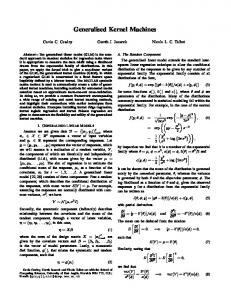
Figure 1: Growth in the CPU and GPU speeds over the last 6 years on benchmarks (Image from [12]) In November 2006, NVIDIA introduced Compute Unified Device Architecture (CUDA)[12], a parallel programming model that leverages the parallel compute engine in NVIDIA GPUs to solve general purpose computational problems. With CUDA, GPUs can be seen as a bunch of parallel co-processor that can assist the main processor in its computations. The OpenCL initiative seeks to provide a similar non-proprietary API for general purpose GPU computing. Fig. 2 shows how current GPU coprocessors appear to a user through CUDA. Each GPU has a set of multiprocessors, each with 8 processors. All multiprocessors communicate with a global memory, which can be as high as 4GB and a constant memory. More capable GPUs share more multiprocessors and more global memory. The 8 processors in each multiprocessor share a local shared memory and a local set of registers. The instructions in the GPU are designed to be executed as parallel threads on multiple data. Therefore, the computations are organized into grids, which are groups of thread blocks. A thread block is defined as a patch of threads that are executed on a single multiprocessor. A maximum of 512 threads can be housed in a single thread block. Each thread performs its operations independently and halts when a synchronization barrier is reached. While GPUs can do double precision, most advantage is gained on single precision computations, and double precision is advised only when it is absolutely essential for algorithmic correctness. Newer GPUs that are to be released in coming years relax this restriction. In all our experiments in this paper, we have used only single precision computations. The main processor (the host) controls the computations and provides the data on which the GPU (the device) can work on. This data is generally transferred from the host memory to the device’s global memory.
which the kernel sums are evaluated as evaluation points (in line with N -body algorithms, which have a similar computational structure). There are several ways each thread can be designed. One obvious parallelization approach is to assign each thread to process the effect of each source point, another one is to assign each thread to process individual evaluation points independently. If each thread is assigned to evaluate the effects of a particular source on all evaluation points, it would have to update the value at each evaluation point in the global memory, thus requiring a number of global memory writes, resulting in a memory inefficient algorithm. However, if each thread is assigned to evaluate a particular evaluation point, it would require only one global memory write per thread. This would however result in several global reads per thread. In this case the use of shared memory and registers can reduce the number of global accesses. We assign each thread to evaluate the kernel sum on an evaluation point. Suppose there are N source points, each thread would be required to read N source points from global memory. We reduce the total accesses to global memory, by transferring source points to the Figure 2: Logical organization of the GPU memories as shared memory. The shared memory is not large enough seen through CUDA (Image from [12]) to house the entire data. So it is required to divide The global memory is large enough to hold many of the the data into chunks and load them according to the large datasets usually encountered (∼ 4GB on current capacity of the shared memory (the number of source GPUs). It is important to note that access times to points that can be loaded to the shared memory is different memories in the device are significantly differ- limited by its size and data dimension). The size of ent. Accesses to global memory are the most expensive each chunk is set to be equal to the number of threads and it takes approximately 400 clock cycles for one ac- in the block, and each thread transfers one source cess. However, if each thread in a block accesses con- element from the global memory to the shared memory, secutive global memory locations, it takes lesser time thus ensuring coalesced memory reads. The weights than a random access. This is referred as memory coa- corresponding to each source is also loaded to the shared lescing. Accesses from the cached constant and texture memory in the same way. Once the source data is memory, which can be written to from the host, are available in the shared memory, all threads update the cheaper. Read and write local memory is provided by kernel sums involving the source points in the shared shared memory (which is shared between all processors memory. in a multiprocessor), and per-processor register memIn order to further reduce the global memory acory, and takes only as long as one instruction. The key cesses, we use local registers for each evaluation point difference between an efficient algorithm on a sequential and the evaluation sum. Once all the source data are processor and a graphics processor is that the former re- evaluated, the sum in the register is written back to quires to have as less computation as possible while the global memory. The algorithm is summarized in Talatter needs to minimize memory access to and from the ble 1. If d is the dimension of the data points, then global memory. In other words, an efficient GPU algo- we use d + 1 shared memory location per thread (one rithm should ensure a coalesced transfer of data from source point and its kernel weight) and d+1 registers per the global memory to the local shared memory, a paral- thread (one evaluation point and the corresponding kerlelization strategy that results in most of the work being nel sum). The proposed approach is generic and can be done on data that is in local registers or shared memory, extended to any kernel, an important distinction from and a well defined patterns of access to global memory. the CPU based approximation algorithms [8, 24, 16, 11]. Accelerating iterative algorithms: Several kernel 3 Accelerating kernel methods on GPUs machines involve solution of linear or least square sysKernel summation: We will refer to the data points tems with kernel matrices, or computation of a few xi in Eq. (1.1) as source points, and the points at
GPU based acceleration for kernel summation Data: Source points xi , i = 1, . . . , N , evaluation points yj , j = 1, . . . , M Each thread evaluates the sum corresponding to one evaluation point: Step 1: Load evaluation point corresponding to the current thread in to a local register. Step 2: Load the first chunk of source data to the shared memory. Step 3: Evaluate part of kernel sum corresponding to source data in the shared memory. Step 4: Store the result in a local register. Step 5: If all the source points have not been processed yet, load the next chunk, go to Step 3. Step 6: Write the sum in the local register to the global memory. Table 1: Data-parallel kernel summation on the GPU eigenvalues and eigenvectors of a kernel matrix. Iter- The proposed approach is summarized in Table 2, where ative approaches are used for problems of this type. we use “mat-decomp” to denote the algorithms in [23]. These include conjugate gradients [6] for Gaussian pro- We load a chunk of the training and test points to the cess regression, power iterations for eigenvalue compu- shared memory and generate the block of the kernel tations, more sophisticated Krylov and Arnoldi meth- matrix that involving these training/test points in the ods, and others. In each case, the core computation per current thread block. This is repeated across all the iteration is the matrix vector product, with the compu- thread blocks to construct the entire kernel matrix, tation of a residual or error term. We discuss individual which can be used for matrix decomposition. cases in the experimental section. As far as GPU im- 4 Experiments plementations are concerned, accelerations are achieved by having the above sum evaluated in the iterative pro- We tested the GPU accelerated kernel methods with cedure. Better speedups can be obtained if the data be- three classes of problems. The first problem class tween iterations are allowed to stay on the GPU, thus used the accelerated summation on different kernels and avoiding data transfers between host and device. The tested the speedup on a synthetic data. Further we other way to accelerate these algorithms is to reduce extended our approach to speed-up kernel density estithe number of iterations via techniques such as precon- mation. We also compare GPU based Gaussian kernel ditioning. GPU implementation of these are subject of summation with a linear algorithm, FIGTREE [11]. In the second problem class, we looked at different itercurrent research. Accelerating kernel matrix decompositions: ative approaches which employ the kernel summation Several matrix decompositions are already available on over each iterations. Finally we look at algorithms that use kernel matrix decompositions and accelerate them the GPU [23] and here, the strategy is to use CPU algorithms, with part of the computation performed on using our acceleration (Table 2). the GPU. To accelerate kernel methods, these libraries Host and device: In all experiments the host procescan be used as is, similar to the way Lapack and other sor is an Intel Xeon Quad-Core 2.4GHz with 4GB RAM. libraries are used to accelerate CPU versions of kernel The GPU is a Tesla C1060 which has 240 cores arranged methods. Given the training and test data, the kernel as 30 multi-processors. It has 4GB of global memory, 16384 registers per thread block and 16kB shared memmatrix needs to be constructed before decomposition. Constructing the matrix has a computational complex- ory per multiprocessor. For all experiments, GPU codes were written in ity of O(dN 2 ) in most kernels, d being the dimension CUDA and compiled with Matlab linkages. Similarly, of the input data. For higher dimension (d > 50) the the CPU codes were written in C++ with Matlab matrix construction cost can become as significant as linkages. This allowed for convenient execution of the decomposition itself, because of the availability of machine learning algorithms. optimized implementations of the decomposition algorithms. However, if the structure of the kernel matrices 4.1 Experiment1 - Kernel summations: We acis utilized, the matrix construction can also be paral- celerated widely-used kernels namely the Gaussian (Eq. lelized on the GPU. Notice that, the matrix decompo- 4.2), Matern (Eq. 4.3), periodic (Eq. 4.4) and Epanechsitions return a matrix which requires O(N 2 ) memory, nikov (Eq. 4.5) kernels given by, � � and memory requirements in these approaches cannot (d(xi , x))2 , be reduced by generating the kernel matrices on-the-fly (4.2) K(xi , x) = s × exp − 2 as in the kernel summation. √ √ We construct the matrix on the GPU and utilize (4.3) K(xi , x) = s×(1+ 3d(xi , x))×exp(− 3d(xi , x)), this matrix for decomposition using approaches in [23]. (4.4) K(xi , x) = s × exp (−2 sin2 (π ∗ d(xi , x))),
Accelerated kernel matrix construction for matrix decomposition Data: Source points xi , i = 1, . . . , N , evaluation points yj , j = 1, . . . , M Each thread evaluates one element of the kernel matrix Step 1: Load the source points from global memory into the shared memory. Step 2: For large data dimension which can not fit into shared memory, divide the each source vector into several chunks of constant size and load them consecutively. Step 3: Compute the distance contribution of the current chunk in a local register, and load the next chunk. Repeat this until the complete dimension is spanned. Step 4: Use the computed distance for evaluating the matrix entry. Step 5: Write the final computed kernel matrix entries into global memory. Step 6: Use the kernel matrix with mat-decomp Table 2: Our accelerated kernel construction using the GPU for matrix decomposition riodic/Gaussian. This can be attributed to the fact that for simpler kernels, the data transfer time is more dominant than for a complex kernel. As the dimension increases, the number of threads that can be accommodated on each processor is reduced to fit the data in the shared memory, and hence there is a reduction in the speedup. Comparison with FIGTREE: There are several approximation algorithms that evaluate the kernel summations in linear time, for example, FIGTREE [11] for the Gaussian kernel. Inspite of the speedups obtained by the GPU-based approach, the asymptotic dependence on data size is still O(N 2 ). Therefore, a linear approach like FIGTREE [11] will outperform it at some point. In order to explore this, we compared the performance of our GPU algorithm with FIGTREE Figure 3: Speedup obtained on a GPU for various which combines two popular linear approximation algokernel summations for a data size of 10, 000. The rithms, Improved Fast Gauss Transform (IFGT) [24, 16] mean absolute error between the CPU and GPU based and tree based approaches, and automatically chooses the fastest method for a given data. We expected summation in all the cases were less 10−5 . FIGTREE to beat our implementation at some point, this was observed only for a data size greater than (4.5) K(xi , x) = s × (1 − d(xi , x)2 ) × 1(d(xi , x) < 1), 128, 000 as seen in Fig. 4a. where d(xi , x) is the Euclidean distance between the Although, the linear approach eventually outperpoints xi and x, s is a scaling parameter and 1(d(xi , x) < forms the GPU version, the performance of these ap1) is an indicator function. Also there is a bandwidth h proaches are found to have great dependence on data diassociated with distance d(., .) such that, mensions and kernel bandwidth. Also, these approaches d are restricted to the Gaussian kernel and require a fixed 2 X kx1,k − x2,k k bandwidth over the data. In contrast, our GPU based (4.6) d(x1 , x2 ) = . h2 approach can be used with any kernel for varying bandk=1 widths. We compared the performance of our algorithm The synthetic data for this experiment were genwith FIGTREE for various dimensions and kernel banderated by choosing a random number between 0 and 1 widths and the results are shown in Fig. 4b and Fig. uniformly for each dimension of the source and eval4c. While the GPU approach performs consistently uation points. Datasets of varying dimensions are across bandwidths, the automatically tuned approach generated in this fashion. The resulting speedup for has varying performances across bandwidths. It was each kernel for a 10, 000-size data is shown in Fig. 3. also observed that the speedup obtained by the GPU The speedup obtained is lower for a simple kernel like approach over FIGTREE increases with data dimenEpanechnikov, but as the complexity of the kernel insions. creases, the speedup obtained is significant, like for pe-
(a) Across data size
(b) Across bandwidth
(c) Across dimensions
Figure 4: Speedups obtained on the Gaussian kernel compared to FIGTREE[11], the linear algorithm Mean Mean Mean Mean Mean Mean
CPU time for Gaussian kernel GPU time for Gaussian kernel absolute error between estimates CPU time for Epanechnikov kernel GPU time for Epanechnikov kernel absolute error between estimates
25.144s 0.022s ∼ 10−7 25.117s 0.011s ∼ 10−7
Table 3: Performance of kernel density estimation on the 15 normal mixture densities in [10] for a data size of 10000
Figure 5: An example of mean shift clustering on a color image Left: Original Image; Right: Segmented image
Mean CPU time 390.847s Kernel Density Estimation (KDE): KDE (or Mean GPU time 0.369s Parzen window based density estimation) is a nonMean abs error < 10−5 parametric way of estimating the probability density function of a random variable. Given a set of obser- Table 4: Performance on the optimal bandwidth estimavations D = {x1 , x2 , · · · , xN }, the density estimate at a tion problem on the 15 normal mixture densities in [10] new point x is given by, for a data size of 10000 ascent to speed up the mean shift clustering approach in [4]. For the image in Fig. 5, it was observed that the naive direct implementation took almost 13.5 hours, whereas the corresponding GPU implementation took Two kernels widely used for density estimation are only 35s for clustering. the Gaussian kernel (Eq. 4.2) and the Epanechnikov Optimal Bandwidth Estimation: Determining the kernel (Eq. 4.5). We performed KDE based on GPU bandwidth h of the kernel in density estimation is acceleration on the 15 normal mixture densities in [10] of paramount importance for the performance of the and compared performance with a direct approach. The estimator [19]. For a Gaussian kernel, there have been −6 error between the two approaches was less than 10 for several approaches to evaluate the optimal bandwidth each distribution. The results are tabulated in Table 3. for a given data points. We looked at the plug-in 4.2 Experiment2 - Iterative approaches using approach in [18] and accelerated it using the GPU. The kernel summations: In this experiment, we explored key computation in the bandwidth selection approach different algorithms, that uses the kernel summation in [18] is the evaluation of a weighted sum of the (Eq. 1.1) within an iterative algorithm like conjugate GaussianDerivative kernel, gradient. � � (d(xi , x))2 Mean Shift Clustering: Mean shift clustering [4] is (4.8) K(xi , x) = s×Hr (d(xi , x))×exp − , a non-parametric clustering approach based on kernel 2 density estimation. It involves running a gradient ascent over the kernel density estimate in order to where Hr is the rth Hermite polynomial. We used a move each data point towards the local mode. Finally, GPU based GaussianDerivative kernel summation with it returns the set of modes (centers) to which each data a Levenberg-Marquardt based non-linear least point converges. A typical result of mean-shift based squares to solve for the bandwidth of the Gaussian clustering on an image is shown in Fig. 5. kernel like in [18] and the results are shown in Table 4. In this experiment, we apply our approach based Gaussian Process Regression: Gaussian process density estimates over each iteration of the gradient regression is a probabilistic kernel regression approach N
1 X (4.7) f (x) = K N h i=1
�
x − xi h
�
.
Dataset
dxN
Diabetes Abalone Bank7FM CompAct PumaDyn8NH Stock
2x43 7x4177 8x4499 22x8192 8x4499 9x950
CPU Time (s) 0.0473 235.8 631.2 1884.2 467.69 13.34
GPU Time (s) 0.1639 0.79 2.19 9.3 1.72 0.27
Table 5: Performance on Gaussian process regression with standard datasets; d denotes the input dimension and N the size of the input data. The mean absolute error in each case was less than 10−5 for a the Gaussian covariance (kernel) (Eq. 4.2) which uses the prior that the regression function (f (X)) is sampled from a Gaussian process. For regression, it is assumed that a set of datapoints D = {X, y}N i=1 , where X is the input and y is the corresponding output. The function model is assumed to be y = f (x) + � where � is a Gaussian noise with variance σ 2 . Rasmussen et al. [15] use the Gaussian process prior with a zero mean function and has a covariance function defined by a kernel K(x, x0 ) which is the covariance between x and x0 , i.e. f (x) ∼ GP (0, K(x, x0 )). They show that with this Gaussian process prior, the posterior of the output y is also Gaussian with mean m and covariance V given by, m = k(x∗)T (K + σ 2 I)−1 y V = K(x∗ , x∗ ) − k(x∗ )T (K + σ 2 I)−1 k(x∗ ) where x∗ is the input at which prediction is required and k(x∗) = [K(x1 , x∗), K(x2 , x∗) . . . , K(xN , x∗). Here m is the prediction at x∗ and V the variance estimate of prediction. Some popular kernels used with Gaussian process regression are Gaussian (Eq. 4.2), Matern (Eq. 4.3)and periodic kernels (Eq. 4.4). The parameters of the kernels s and h are called the hyperparameters of the Gaussian process and there are different approaches to estimate these [15]. Given the hyperparameters, the core complexity in Gaussian processes involves solving a linear system involving the kernel covariance matrix and hence is O(N 3 ). Gibbs et al. [6] suggest a conjugate gradient based approach to solve the Gaussian process problem in O(kN 2 ), k being the number of conjugate gradient iterations. Over each iteration of the conjugate gradient, the key computation is a weighted summation of the covariance kernel functions. In this experiment, we used our GPU based kernel summation to speed up each iteration of the conjugate gradient. Table 5 shows the performance of Gaussian process regression on various standard datasets [22] for a Gaussian kernel.
Learning a Ranking function: In information retrieval, a ranking function is a function that ranks data matching a given search query point according to their relevance. In order to rank the data, a preference relation needs to be learned, which is given by the ranking function. A ranking function f maps a pair of datapoints to a score value, which can be sorted for ranking. There are several approaches to learn the ranking function for a given dataset. We particularly looked at the preference graphs based approach in [17]. Raykar et al. [17] maximize the generalized Wilcoxon-Mann-Whitney (WMW) statistic [14] using a non-linear conjugate gradient approach to learn the ranking function. Instead of maximizing the WMW statistic, they use a continuous surrogate based on the log-likelihood, thus maximizing a relaxed statistic. They use a sigmoid function to model the pair-wise probability, and approximate it using a erfc function. They thus reduce the core computation of the ranking problem to the evaluation of a weighted sum of erfc functions. A linear algorithm for the summation of the erfc functions is proposed in [17], which is then used for the efficient learning of the ranking function. We use GPU based summation of erfc functions for learning the ranking function and compare it with the linear approach in [17] on the datasets used in [17] and the results are shown in Table 6. We also report the absolute error in the WMW statistic evaluated on the training and testing data, based on the ranking functions learnt from the approach in [17] and our GPU based approach. It can be seen that our approach consistently outperforms the approach in [17]. Note that the approach in [17] is linear in computational complexity, whereas our approach is quadratic and still outperforms the linear approach for large datasets. 4.3 Experiment3: Matrix decompositions Often, in many algorithms, it is required to perform LU, QR or Cholesky decomposition of the kernel matrices, for example [2] and a direct decomposition will have a cubic complexity. The GPU-based summation cannot be used in these scenarios, but however there are many algorithms for performing efficient matrix decompositions accelerated on GPUs. In this experiment, we discuss these approaches for kernel matrices. Volkov et al. [23] claim that their implementation is the fastest LU, QR and Cholesky decomposition as of 2008. We adapted their approach for kernel matrices in this experiment. As the dimension of the input data increases, the construction of the kernel matrices becomes the dominant part of the decomposition, due to the high efficiency of these algorithms. In order to illustrate this, we performed Cholesky and QR decompositions of kernel matrices for data of various dimen-
Dataset Auto California Housing CompAct Abalone
dxN
Raykar [17]
GPU
8x392 9x20640 22x8192 8x4177
0.7499s 105.2s 5.67 9.838s
0.5280s 27.82s 5.56s 5.003s
Error in WMW on training data 0.000 0.003 0.000 0.020
Error in WMW on test data 0.000 0.003 0.003 0.020
Table 6: Performance of WMW-statistic based ranking, GPU based approach vs the linear algorithm in [17], error reported is the total error on the WMW statistic DataSize Direct GPU 1000 0.61s 0.2830s 2500 4.41s 2.1337s 5000 22.06s 12.467s 7500 60.30s 37.28s Table 7: SRKDA [2] - Comparison between the GPU implementation and a CPU implementation on Caltech101 dataset [5]; Mean absolute error (measured on the projection of a test data of size 100) in each case was ∼ 10−5 as a spectral regression and have proposed a spectralregression based KDA (SRKDA). At the core of SRKDA Figure 6: Speedup obtained for Cholesky and QR decom- is a Cholesky decomposition of the kernel matrices, this position of a Gaussian kernel matrix, based on [23] on has resulted in a 27 times theoretical speedup of SRKDA a 10, 000-size data (size of the kernel matrix) for vari- over KDA. However, the Cholesky decomposition remains the ous dimensions of the input data; the speedups reported here are for the matrix construction on GPU us- core computational task of SRKDA, and its cubic ing Table 2 and decomposition using [23] against complexity is still computationally expensive for large the matrix construction on CPU and GPU de- datasizes. We address this problem using the proposed composition using [23]. The mean absolute error in kernel matrix decomposition. We performed SRKDAbased decomposition on the SIFT features extracted each case was less than 10−4 . from the 10 classes of the CalTech-101 dataset [5]. The results are tabulated in Table 7. It is evident that sions for a 10, 000-size synthetic data (generated as be- there is a significant improvement in the performance fore). We decomposed a Gaussian kernel matrix on the compared to a direct implementation. GPU using [23], compared the performance for the matrix constructed on the CPU with the GPU counterpart, 5 Conclusions and the results are shown in Fig. 6. As the data dimen- In this paper we have looked at accelerating popular sion increases, the speedup obtained also increases. This kernel approaches using the GPU. We have reported suggests that for large dimensions, matrix construction the speedups obtained for the summation and decomtakes significant time and hence the proposed approach position of various kernels on GPUs. Our approaches would increase speedup. are not just limited to the kernels reported and can be Spectral Regression for Kernel Discriminant extended to any generic kernel. Further, we have shown Analysis: Linear discriminant analysis (LDA) is a the improvement in performance in different kernel mastatistical projection approach, where the projections chines like kernel density estimation, Gaussian process are obtained by maximizing the inter-class covariance, regression, learning a Ranking function and kernel diswhile simultaneously minimizing the intra-class covari- criminant analysis using spectral regression. We have ance. For non-linear problems, the LDA is performed on also compared our performance with a linear algorithm the kernel space and is termed as Kernel discriminant [11]. With the increasing speeds in GPUs compared to analysis (KDA). KDA requires the eigen decomposition the CPUs (as shown in Fig. 1), the performance can of the kernel matrix and hence is computationally ex- only improve further and can provide effective solution pensive for large datasizes. Cai et. al [2] address this to computation bottlenecks in various kernel machines. problem by casting the eigen decomposition problem We have made these algorithms in CUDA with Matlab
linkages available under LGPL as an opensource1 and we hope to keep evolving the library. Possible areas of improvement include the following. Accelerating linear algorithms: In Section 4.1, we compared our implementation with a linear version of Gaussian kernel summation. It was evident that inspite of the speedup obtained by our approach, a linear algorithm will eventually beat it. Motivated by this, we tried to map parts of the linear algorithm in [11] on the GPU and achieved speedups up to 3X for some stages. The chief bottle-neck here is the construction of underlying data-structures and if there can be an appropriate map of the data structures to the GPU, the speed up can be substantially increased like in [7]. Accelerating kernel summation for higher dimensions: The proposed approach for kernel summation is limited by the size of the shared memory of the graphics processor. Thus, for very large dimensions (> 2000), it is impossible to house even one datapoint in shared memory. While it is still possible to use the GPU to improve the performance by using all the data from the global memory, this approach will be suboptimal. This is particularly interesting in the context of problems with a large number of training and test points, with each point in a very high dimensional space. References [1] C. Bishop, Pattern Recognition and Machine Learning (Information Science and Statistics), Springer-Verlag New York, Inc., 2006. [2] D. Cai, X. He, and J. Han, Efficient kernel discriminant analysis via spectral regression, in IEEE International Conference on Data Mining, IEEE Computer Society, 2007, pp. 427–432. [3] B. Catanzaro, N. Sundaram, and K. Keutzer, Fast support vector machine training and classification on graphics processors, in International Conference on Machine Learning, 2008, pp. 104–111. [4] D. Comaniciu and P. Meer, Mean shift: a robust approach toward feature space analysis, IEEE Transactions on Pattern Analysis and Machine Intelligence,, 24 (2002), pp. 603–619. [5] L. Fei-Fei, R. Fergus, and P. Perona, Learning generative visual models from few training examples: An incremental Bayesian approach tested on 101 object categories, 2004, p. 178. [6] M. Gibbs and D. Mackay, Efficient implementation of Gaussian processes, tech. rep., 1997. [7] N. Gumerov and R. Duraiswami, Fast multipole methods on graphics processors, Journal of Computational Physics, 227 (2008), pp. 8290–8313. 1 www.umiacs.umd.edu/users/balajiv/GPUML.htm
[8] D. Lee, A. Gray, and A. Moore, Dual-tree fast Gauss transforms, in Advances in Neural Information Processing Systems 18, 2006, pp. 747–754. [9] S. Lukasik, Parallel computing of kernel density estimates with MPI, in International conference on Computational Science, Springer-Verlag, 2007, pp. 726–733. [10] J. Marron and M. Wand, Exact mean integrated squared error, The Annals of Statistics, 20 (1992), pp. 712–736. [11] V. Morariu, B. Srinivasan, V. Raykar, R. Duraiswami, and L. Davis, Automatic online tuning for fast Gaussian summation, in Advances in Neural Information Processing Systems, 2008. [12] NVIDIA, NVIDIA CUDA Programming Guide 2.0, 2008. [13] J. Ohmer, F. Maire, and R. Brown, Implementation of kernel methods on the GPU, in Digital Image Computing: Technqiues and Applications,, Dec 2005, pp. 543–550. [14] G. Omer, R. Rosales, and B. Krishnapuram, Learning rankings via convex hull separation, in Advances in Neural Information Processing Systems, 2006, pp. 395–402. [15] C. Rasmussen and C. Williams, Gaussian Processes for Machine Learning, The MIT Press, 2005. [16] V. Raykar and R. Duraiswami, The improved fast Gauss transform with applications to machine learning, in Large Scale Kernel Machines, 2007, pp. 175–201. [17] V. Raykar, R. Duraiswami, and B. Krishnapuram, A fast algorithm for learning a ranking function from large-scale data sets, IEEE Transactions on Pattern Analysis and Machine Intelligence, 30 (2008), pp. 1158–1170. [18] S. Sheather and M. Jones, A reliable data-based bandwidth selection method for kernel density estimation, Journal of the Royal Statistical Society, 53 (1991), pp. 683–690. [19] B. Silverman, Density Estimation for Statistics and Data Analysis, Chapman & Hall/CRC, April 1986. [20] D. Steinkraus, I. Buck, and P. Simard, Using GPUs for machine learning algorithms, in International Conference on Document Analysis and Recognition,, vol. 2, Sep 2005, pp. 1115–1120. [21] D. Thanh-Nghi and V. Nguyen, A novel speed-up SVM algorithm for massive classification tasks, July 2008, pp. 215–220. [22] L. Torgo. Available at http://www.liaad.up.pt/ ∼ltorgo/Regression/DataSets.html. [23] V. Volkov and J. Demmel, LU, QR and Cholesky factorizations using vector capabilities of gpus, Tech. Rep. UCB/EECS-2008-49, EECS Department, University of California, Berkeley, May 2008. [24] C. Yang, C. Duraiswami, and L. Davis, Efficient kernel machines using the improved fast gauss transform, in Advances in Neural Information Processing Systems, 2004.