Grasp Recognition for Uncalibrated Data Gloves: A Machine Learning

Guido Heumer* Heni Ben Amor Bernhard Jung VR and Multimedia Group Institute of Informatics TU Bergakademie Freiberg Bernhard-von-Cotta Strasse 2 09599 Freiberg, Germany

Grasp Recognition for Uncalibrated Data Gloves: A Machine Learning Approach

Abstract This paper presents a comparison of various machine learning methods applied to the problem of recognizing grasp types involved in object manipulations performed with a data glove. Conventional wisdom holds that data gloves need calibration in order to obtain accurate results. However, calibration is a time-consuming process, inherently user-specific, and its results are often not perfect. In contrast, the present study aims at evaluating recognition methods that do not require prior calibration of the data glove. Instead, raw sensor readings are used as input features that are directly mapped to different categories of hand shapes. An experiment was carried out in which test persons wearing a data glove had to grasp physical objects of different shapes corresponding to the various grasp types of the Schlesinger taxonomy. The collected data was comprehensively analyzed using numerous classification techniques provided in an open-source machine learning toolbox. Evaluated machine learning methods are composed of (a) 38 classifiers including different types of function learners, decision trees, rule-based learners, Bayes nets, and lazy learners; (b) data preprocessing using principal component analysis (PCA) with varying degrees of dimensionality reduction; and (c) five meta-learning algorithms under various configurations where selection of suitable base classifier combinations was informed by the results of the foregoing classifier evaluation. Classification performance was analyzed in six different settings, representing various application scenarios with differing generalization demands. The results of this work are twofold: (1) We show that a reasonably good to highly reliable recognition of grasp types can be achieved— depending on whether or not the glove user is among those training the classifier— even with uncalibrated data gloves. (2) We identify the best performing classification methods for the recognition of various grasp types. To conclude, cumbersome calibration processes before productive usage of data gloves can be spared in many situations.

1

Introduction

A desirable goal for many applications of immersive VR is the support of natural virtual object manipulations that closely resemble the manipulation of real objects. Natural object manipulations are, for example, fundamental in virtual prototyping for accurate simulation of the operation or assembly of virPresence, Vol. 17, No. 2, April 2008, 121–142 ©

2008 by the Massachusetts Institute of Technology

*Correspondence to [email protected].

Heumer et al. 121

122 PRESENCE: VOLUME 17, NUMBER 2

tual product models (Zachmann & Rettig, 2001). Similarly, the imitation of a VR user’s manipulation of virtual objects has been proposed as a means for programming assembly robots by demonstration (Aleotti & Caselli, 2006) and for generating virtual character animations that faithfully reproduce the user’s interactions with scene objects (Jung, Amor, Heumer, & Weber, 2006). To support such natural manipulations, it is crucial that the VR system is able to differentiate between various types of human grasping. VR-based manipulations of virtual objects are commonly facilitated through data glove-type input devices, such as Immersion’s Cyberglove. In order to recognize a user-performed grasp, the sensor readings of the data glove have to be processed, analyzed, and matched to one of a set of known grasp types. Typically, before using the data gloves, a time-consuming calibration phase is needed in order to account for differences in hand size and proportion when mapping from raw sensor readings to joint angles of the user’s hand. How an optimal calibration can be achieved is still an unsettled question. The more accurate methods rely on external vision systems, which themselves need to be calibrated. Due to the complicated procedure, an accurate calibration of data gloves is often not possible, particularly in settings that demand immediate availability for new user groups, such as public installations. A main motivation for the work described here is therefore to find out whether it is possible to recognize a range of hand shape types during manipulations directly from raw sensor input without the intermediate joint angle representations. If successful, the cumbersome calibration phase could be spared, enabling an immediate productive use of data gloves in immersive VR systems in many situations where reliable classification of hand shapes (rather than exact reconstruction of joint angle values) is sufficient for the application. A second motivation for this work is to evaluate the performance of different classification methods. The aim is to identify the classifier (or combination of classifiers) that is best suited for the problem domain of grasp recognition from raw data glove sensor data. One justification for this endeavor results from the so-called “no free lunch” (NFL) theorems in machine learning (Wolpert

& Macready, 1997). The NFL theorems state that averaged over all possible problems, all learning algorithms perform equally. As a consequence, there cannot be one classification technique that is optimal for all classification tasks. However, when restricting the classification problem to a particular domain, there might well be a classifier (or a combination of classifiers) that outperforms all others. This leads to the conclusion that selecting a good classifier should be based on an empirical evaluation in the respective problem domain. Following this reasoning, we systematically evaluated a wide range of machine learning techniques for this problem domain. We have experimented with a total of 38 standalone classifiers, five meta-classifiers each combining several base classifiers, and principal component analysis for dimension reduction as a data preprocessing step in various settings to find out which classifiers are suited best for this type of problem. The settings reflect different possible use-cases and application scenarios. In this way, informed decisions can be made about whether or not to use a particular classification method in a given VR scenario.

2

Related Work

A variety of research in the fields of medicine, robotics, developmental psychology, and VR has led to the formulation of grasp taxonomies: categorizations of grasps based on form or function. An early taxonomy is described in Schlesinger’s work on constructing artificial hands (Schlesinger, 1919). He characterized which functionalities in prosthetic hands are needed to grasp certain objects. Building on this work, Taylor and Schwarz (1955) defined English names for the most important grasps investigated by Schlesinger: cylindrical, tip, hook, palmar, spherical, and lateral grip (see Figure 1 for examples). Napier researched the basic task requirements of grasps and differentiated between two basic grasp types: the power grip, which clamps an object firmly under usage of the palm, and the precision grip, where the thumb and other fingers pinch the object (Napier, 1956). Later, Cutkosky investigated opti-

Heumer et al. 123

mal grasp operations in factories and developed a taxonomy for categorizing feasible grasp types in this domain (Cutkosky, 1989). In order to enable the computer to recognize and match a user-performed grasp onto a corresponding class from the taxonomy, techniques from the area of pattern classification can be applied. In Friedrich et al. (1999), a neural network classifier and the Cutkosky taxonomy were used for this purpose, yielding a classification rate of about 90% for grasps performed using a data glove. According to Ekvall and Kragic (2005), a hidden Markov model (HMM) based method was even able to achieve recognition rates of close to 100% for single user settings. However, recognition rates dropped significantly (to about 70%) for settings with multiple users. In Aleotti and Caselli (2006), a nearest neighbor classifier is used in conjunction with heuristic rules. The task of these rules is to disambiguate between similar grasps. In this way, recognition rates of 94% for seen users (those users who trained the system) and 82% for unseen users (those users who worked with the system but did not run the system themselves) were achieved. Applying a classifier to unseen users always bears the risk of significantly lower recognition rates. This stems from the fact that even identical postures can produce different sensor values when the sizes of the subjects’ hands vary. One way to tackle this problem is to perform a calibration process as in Kahlesz, Zachmann, and Klein (2004). However, this process can be complex, timeconsuming, and in itself error-prone. In a recent paper by Borst and Indugula (2005) on realistic virtual grasping, it was noted that even time-consuming calibration procedures do not produce accurate results. Another way to solve this problem is to use classification algorithms that are able to generalize over a large set of users. However, it is still an open issue which classification techniques can achieve such generalization as no thorough comparison has been conducted so far. Another interesting question that needs further investigation is the performance of classification techniques in different application scenarios; for example, applications where new objects are grasped vs. applications where the size and shape of all objects are known in advance. In contrast to previous research, the work presented

in this paper does not focus on a particular classification algorithm or a particular setting. Instead, we try to compare the performance of a wide range of classifiers in several settings within the domain of grasp classification. Such a comprehensive evaluation enables us to draw various conclusions about the applicability and the success of classification with uncalibrated data gloves.

3

Data Acquisition

In the data acquisition phase of our study, sensor value data was captured from several users, performing all the grasps of Schlesinger’s taxonomy (Schlesinger, 1919) on various real objects. After recording the raw data, a first analysis was done on the basis of a Sammon mapping of a self-organizing map (Kaski, 1997). The experimental setup and the results of the data analysis are presented after a short illustration of how the hand posture is measured by the type of data glove used.

3.1 Data Glove The data glove used for recording was a 22-sensor wireless Cyberglove 2 by Immersion, Inc. (see Figure 1). This type of data glove measures hand posture through a number of resistive bend-sensing sensors that are placed in key locations (mostly joint positions) on a stretch fabric glove. Each of the sensors measures its amount of bending around one axis (the flat side) in the form of an 8-bit value between 0 and 255, which is almost linearly proportional to the bend angle. It is important to note that the measured sensor values do not directly represent finger joint angle values. For the mapping from sensor values to actual joint angles, a complex calibration and conversion process is necessary that involves several pitfalls. In the easiest case of measuring the flexion of the interphalangeal joints, a direct linear conversion from one sensor value to a joint angle can be performed. This involves an offset value (sensor value for which the joint angle is zero) and a gain factor (a multiplicative term to convert the bend value to rad/deg). Even for this simplest method of


Table 1. The Grasp Types and Corresponding Trial Objects Grasp type

Objects

Cylindrical Hook Lateral Palmar

Bottle, hammer, flower pot, coffee jug Plastic case, toolbox, backpack, bag Floppy disk, key, ID card, CD case Small box, matchbox, tape roller, PDA case Tennis ball, egg-shaped case, bowl, mouse Nail, pencil, small eraser, PDA top

Spherical Tip

mapping, offset and gain values have to be determined for each single sensor in a tedious process. The situation becomes even more complicated for joints that have more than one degree of freedom and thus influence more than one sensor. Due to cross-couplings between the sensors, more complex forms of calibration are necessary to achieve a satisfactory fidelity. In Kahlesz et al. (2004), some recent calibration techniques are summarized. Since our objective was to spare any calibration process, the raw sensor readings, as transmitted by the Cyberglove 2, were used directly as a feature vector for hand posture classification.

3.2 Experimental Setup For each of the six grasp types, four objects of various shapes were grasped. The objects were chosen in such a way that each object naturally affords one of the Schlesinger grasp types. Table 1 lists the objects used for each grasp type, and Figure 1 shows pictures of some of these objects. For each object, two trial sequences were performed. In the first sequence, the object was grasped five times, with the participant’s grasping hand starting from a fixed position on the table. During this whole sequence the participant sat at the table. In the second sequence, the object was again grasped five times. This time, however, the hand starting position was varied randomly, as was the object’s orientation on the table. For larger objects, like the tool box, the participating user was stand-

ing during this sequence. The captured data consisted of all the 22 glove sensor values representing the hand posture at the “peak” moment of the grasp—as opposed to a sequence of sensor values of a full grasping movement. This moment means the time the participant’s hand firmly held the object and the fingers were at rest. The peak moment was determined manually by pressing a button on the data glove. The whole data acquisition process was conducted with six participating users. Each user was adult, male, and right-handed. In total, 6 (participants) ⫻ 24 (objects) ⫻ 10 (grasps per participant and object) ⫽ 1,440 data items were collected.

3.3 Data Visualization Before the classifier evaluation was executed, it proved interesting to first take a “glimpse” at the data. This helped to get an idea of the problem difficulty, to assess the quality of the recorded data, and to gain first ideas about hard-to-differentiate grasp types. Typically, the recorded data is in a higher-dimensional space—in the case of our data glove a 22-dimensional space— which makes human inspection difficult. For inspection and analysis purposes it is more convenient to create a visual representation of the experimental data. This can be achieved through a projection of the high-dimensional pattern space onto two dimensions. Common techniques for such projection tasks are the self-organizing map and Sammon mapping (Kaski, 1997). Figure 2 shows a projection of our experimental data using a combination of the two techniques. The projection is distance preserving, which means that points which are close to each other in the higher dimensional space will also be close to each other in the projection. It can be seen that the spherical grasp forms a particular region in the upper part of the map. This region can neatly be separated from regions representing other grasps, which indicates that classification of spherical grasps is particularly easy. Although other grasp types also occupy particular regions on the map, they are much more intermixed. This yields complex decision boundaries. For example, the classes tip and palmar cannot be cleanly separated from each other. What also be-

Heumer et al. 125

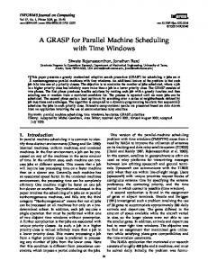
Figure 1. Images of some of the objects used during the grasping experiments with their corresponding grasp types.

Figure 2. Sammon mapping of a self-organizing map representing the data projected onto a two-dimensional space.

comes visible is that cylindrical grasps are scattered throughout the map. This observation is particularly interesting, as it exemplifies the hard separability of the Schlesinger grasps based on hand shape only. Specifically, we can expect classification to be more error-prone for cylindrical grasps and that some grasp types, such as palmar and tip, could be especially hard to distinguish.

4

Classifier Evaluation

A set of 38 different classifiers from the freely available Weka data mining software package (Witten & Frank, 2005) has been evaluated. If not stated otherwise, all classifiers were run in an “out of the box” fashion, that is, with default settings and without any pa-


rameter optimization. The examined algorithms can be broadly divided into five categories—probabilistic methods, function approximators, lazy learners, trees, and rule sets. 1. Probabilistic methods such as the naive Bayes classifier (Friedman, Geiger, & Goldszmidt, 1997) or Bayes nets (Cooper & Herskovits, 1992) learn to discriminate between classes by building probability models of each class. Using Bayesian inference, the probability of a new data item belonging to a particular class can be computed. For example, the naive Bayes classifier learns a model of the training data by estimating class probabilities and conditional probabilities of the variables. Together with the Bayes theorem, these values can be used to compute the probability of a data item belonging to a particular class. The only “naive” assumption (hence the name) that is being made, is that all variables of a data item are mutually independent. 2. Function approximators learn the parameters of a function which takes the new data item as an input and returns the class as an output. Well-known representatives of this type of algorithm are multilayer perceptrons and radial basis networks (Bishop, 1995). Here, the approximated function is represented by a set of interconnected neurons. The back-propagation algorithm (Haykin, 1994) can be used to train such networks in order to minimize the squared error of approximation. More modern variants of this class are support vector machines (SVM; Cristianini & Shawe-Taylor, 2000) and Gaussian processes (GP: Rasmussen & Williams, 2005). A basic concept underlying both SVM and GP is the concept of kernels. Linear combinations of kernels centered around training data points are used for making predictions (Bishop, 2006). This allows the use of the so-called kernel-trick. The basic idea behind the kerneltrick is to replace all dot products by a kernel function that maps the original data into a higher-dimensional space. As a result, it is possible to perform a linear classification in the higher-dimensional space that corresponds to a nonlinear classification in the original space. The choice of a proper kernel function is therefore crucial to successful classification. For SVM we used a polynomial kernel and for GP we used a radial basis function kernel.

3. Lazy learning techniques (Bontempi, Birattari, & Bersini, 2002) postpone any type of learning until a request for classification of a new data item is received. When such a request is received, a database of previously seen examples is searched for a set of examples, which are closest to the new item (with respect to a given distance metric). 4. Tree classifiers, such as decision trees (Quinlan, 1993), try to break up the classification task into a hierarchy of simple decisions at whose end the final decision determines the class. As the name suggests, this hierarchy has the form of a tree whose nodes represent local decisions, while leaves represent the classes. 5. Finally, rule induction methods (Quinlan, Compton, Horn, & Lazarus, 1987) create sets of logical rules for determining the class of a particular item. Ridor, or “ripple down rule” (Richards, 2002), is a representative algorithm from this class. Ridor requires that the data is incrementally supplied to the training set. Data items that conflict with previously learned rules are seen as exceptions. These are then treated by patching the rule locally for the particular item. Another category, namely meta learning techniques (Chan & Stolfo, 1997; Dietterich, 2000; Polikar, 2006), has been examined in a second evaluation stage, guided by the results of the first one. These are techniques such as boosting or bagging that aim to create more powerful classifiers through the combination of several simpler ones. Depending on the algorithm hierarchies, cascades or ensembles of base classifiers are used for classification. Since meta classifiers can be built from essentially arbitrary combinations of simpler classifiers, they are inherently more complicated to evaluate and a large number of choices of base classifiers would have to be looked at to perform a complete evaluation. For this reason, in our evaluation of the meta schemes (see Section 6), we concentrated on the most promising combinations as determined by the evaluation of base classifier schemes. Some of the examined algorithms, mainly function approximators, are originally regression methods which are not directly usable for classification. To use them as classifiers for our study, they were run via the “classification via regression” method of Weka. This method bi-

Heumer et al. 127

Table 2. Investigated Values of the Variable Objects Value

Meaning

Example scenario

Seen

Classifier trained and tested with the same set of objects Classifier trained and tested with different sets of objects

Applications with a given, fixed set of objects, e.g., a tool set Applications where scene objects change or are of modifiable form, e.g., CAD

Unseen

Table 3. Investigated Values of the Variable User Value

Meaning

Example scenario

Individual Group

Classifier trained and tested with a specific user Classifier trained with a group of users and tested with a group member Classifier trained with several users but tested with a user not in the group

Single operator system Work group

Unseen

narizes the classes and builds a regression model for each class.

4.1 Design and Method To determine which classifier is best suited for the domain of classifying raw sensor data, a comprehensive, systematic classifier evaluation was performed. We examined each classification algorithm in six different settings, formed by a permutation of the values of two situational variables (see Tables 2 and 3), putting different generalization demands on the classifiers. One variable (objects) determined whether the objects grasped in the test set were seen, that is, grasp examples with these objects were used for training, versus unseen, where no grasp examples with these objects were used during training. Note that even in the seen case, training and test sets were always disjoint. This means a grasp example used during training was never used for testing as well. However, due to the nature of our data acquisition phase, it can be assumed that in the seen case for each test item a number of rather similar items could be found in the training set.

Public installation, e.g., game

The other variable (user) determined the user group, that is, which set of users’ grasp examples were taken for training. For this variable, three different cases were investigated: individual and group, where training data of only one user or the full group of users, respectively, were used for training and testing; and a third case, unseen, where data of all users except one was used for training, and data of the held-out user was used for testing. The property of disjoint training and test sets also holds true in all three cases. For each of the six settings, several pairs of disjoint training and test sets were generated by splitting the complete data in an adequate way. This was done in one of two ways. One way was by holding out a certain number of randomly chosen data examples, while ensuring that each grasp type, user, and object gets represented by the same amount of data items in the training set (stratification). The other way of splitting was done in a semantic fashion, by, for example, holding out a certain user of the training set and putting only data of this user into the test set. The method of splitting was specific to each setting and is explained in more detail below. Each classifier was trained and tested with each pair


Table 4. Splitting of Data into Test and Training Sets for the Different Settings* Training set

Setting (user, objects)

Data splitting

#1 - individual, seen objects #2 - individual, unseen objects

Six (per user) times six splits of data of one user. Test set—two random examples per object. Six (per user) times eight splits (two series of four) of data of one user. Test set—one random object per grasp type. Six splits—as in #1 but data of all users. Test set—two random examples per object and user. Eight splits as in #2 but data of all users.

#3 - group, seen objects #4 - group, unseen objects #5 - unseen, seen objects #6 - unseen, unseen objects

Six splits (one per user). Test set—all data of one user. Twelve splits (two series of six). Test set—from user splits (as in #5) hold out one random object per grasp type.

Test set

192†

48†

180†

60†

1,152

288

1,080

360

1,200

240

900

60

*For each of the six users an experiment with the given set sizes has been performed and the results have been averaged. †Given number refers to number of data examples per user.

(or data split), and the average rate of correct classifications for each classifier over all these tests was determined. The feature- (or input-) vector for classification consisted of all 22 sensor values which were not weighted. The output of the classifier was an index value, indicating one of the six grasp types. Note that since all data items were taken from valid examples of the different grasp types, there was no rejection class. The right answer was always one of the six Schlesinger grasp types. Classifier performance was measured in the percentage of correct classifications. When two classifiers had the same average performance, the classifier with the smaller standard deviation was considered better. Additionally, for each setting, a set of best classifiers was established by selecting all classifiers that performed not significantly differently than the best classifier. To determine the significance of differences between classifiers, a McNemar’s test was used with p ⬍ .05. For an overview on significance tests for classifier evaluation, see Dietterich (1998). To obtain an additional measure for classifier performance, a stratified 10-fold cross-validation on

the complete data set was performed for each classifier. This is considered a standard method of predicting the error rate of learning techniques (Witten & Frank, 2005). To cross-validate a data set, it is split into k (where k is 10 in this case) subsets. Then, k tests are conducted where the kth subset is used as the test set for the classifier and the other k–1 subsets are used as the training data. The total classification rate is then computed as the average of the classification rates of all k tests. Stratified means that it is ensured that each class is properly represented in the k subsets. The results of the cross-validation were also regarded as part of the overall classifier performance. The number of data splits into test and training set and the respective set sizes per split are summarized for all settings in Table 4. Also, a rough indication of how the test set was formed is given in the middle column. More detail about the settings and the exact method of how test and training set were generated are given in the following subsections. Readers not interested in this level of detail might want to skip to the presentation of results in Section 4.2.

Heumer et al. 129

4.1.1 Individual User, Seen Objects. In this setting, data of only one user is regarded and the same set of objects is used for testing and training. This corresponds to an application, where the system is trained for a specific user (and this user only) and all objects to be interacted with are known in advance. In comparison with conventional (calibrated) classification, this would correspond to a perfect glove calibration being available for a particular user and an additional training session having been performed, where all objects later to be interacted with are trained into the system. To generate disjoint training and test sets for this setting, all data of one user was taken and split evenly into two sets, so that the respective numbers of examples for each grasp and object stayed the same. Since 10 data samples for each object were recorded—five with a fixed starting position and five with a variable starting position—two samples of each object (one with each type of starting position) were chosen for the test set (48 data items), while the others formed the training set (192 data items). Overall, six splits were generated in this way, by randomly choosing the test items. This process has been repeated for each of the users, thus resulting in 6 ⫻ 6 data splits. The performance of the individual user tests was averaged over all users. 4.1.2 Individual User, Unseen Objects. Again, data of only one user is regarded; however, tests were always performed with unseen objects, that is, no data examples of the objects used for the tests have been used for training. This corresponds to an application where the system was trained for a specific user; however, the objects used during the interaction are not previously known. Training and test sets were generated by randomly choosing one object per grasp type and using the examples of these objects as the test set, whereas the data of the other objects was used as the training set. This way, for each user, a series of eight splits was generated, so that each object of one grasp type was used exactly twice for testing. The training sets consisted of 180 data items, whereas the test sets were 60 items. The combinations between grasp types, that is, which object of each grasp type was chosen, were random. It was en-

sured, however, that each permutation only occurred once. As in Section 4.1.1 (individual user, seen objects), the results were averaged over all users. 4.1.3 Seen Group of Users, Seen Objects. Similar to Section 4.1.1 (individual user, seen objects), the difference is that data examples of all users were used for training and testing. This corresponds to an application that is set up to work with a certain group of users and the objects used for interaction are known in advance. Note that this setting, similar to the settings below, is already beyond the scope of calibration-based approaches as it is not necessary to specify which user is currently using the system. Data splitting was done as in the individual user case, but with data of all users instead of one. Additionally, it was ensured that the same number of examples from each user was chosen. For each object and user combination, two examples were randomly held out for the test set (288 data items), while the remaining examples formed the training set (1,152 data items). 4.1.4 Seen Group of Users, Unseen Objects. This setting is similar to Section 4.1.2 (individual user, unseen objects). However, data of all users were used for training and testing instead of data from just one user. This corresponds to an application that is set up to work with a certain group of users and the objects used for interaction are not known in advance. Training and test sets were generated by creating eight splits, wherein each split data of one randomly picked object (per grasp type) forms the test set (360 data items), whereas data from the remaining objects comprises the training set (1,080 data items). Again, it was ensured that no permutation was repeated and that each object was part of the test sets exactly twice. 4.1.5 Unseen Users, Seen Objects. In this setting, all data of the test user was held out of the training set, that is, the classifier did not see any data item from the test user during training. This corresponds to an application where the system was trained with data from a group of users and another (previously unseen user) then uses the system, for example, in public installa-


tions, demo showcases, and so on. All objects used during tests were seen before by the classifier (grasped by other users) during training, that is, for this type of application the objects of the interaction need to be known in advance. Here, for each user a pair of datasets was generated, where the training set contained sensor data from all users except this one (1,200 data items), and the test set consisted of all data from this user (240 data items). Since data was acquired from six different users, this resulted in six different disjoint splits. 4.1.6 Unseen Users, Unseen Objects. In this setting neither the objects nor the user involved in testing were seen by the classifier during training. This corresponds to applications where the users and interaction objects are not known in advance. This setting puts high demands on the classifier’s generalization capabilities, but can satisfy the broadest range of use cases. For generating test sets and training sets, the data was first split into disjoint sets for each user as in Section 4.1.5. Then, for each of these user splits, two random object splits were generated, where for each grasp type one object was picked. Data from this object was removed from the training set, whereas only the data of this object remained in the test set. This resulted in 12 data splits overall with a test set size of 60 data items and a training set size of 900 data items.

is given in milliseconds. This value is of course dependent on the used hardware and for this reason is only to be seen as a relative comparison between the several algorithms. Dark gray table cells indicate for each setting the classifier with the highest accuracy; table cells shaded in light gray indicate classification methods of which the accuracies vary only insignificantly (according to a McNemar’s test) from the best performing classifier. The interested reader can find the complete results of the study as well as the captured data on the Web under http://vr.tu-freiberg.de/grasping/. In the following, the results for each of the settings are summarized. ●

●

4.2 Results For every classification algorithm evaluated in each data split of each setting, the percentage of correctly classified examples has been determined. Due to space limitations this is too much information to be presented here. Hence, the results have been summarized by determining average classification rates for each setting and the corresponding standard deviation, and can be seen in Table 5. Each setting is represented by two columns (average and standard deviation). Following the cross-validation results, in the next two columns are the average performance over all settings and the standard deviation of this total average. In the final column, the average runtime per test of each classification algorithm

●

Individual User, Seen Objects. With 99.48% achieved by the KStar algorithm, a highly reliable classification rate can be reached for the case where the objects grasped are known in advance and the user trained in the system individually. A not significantly worse performance can be obtained with IB1, LibSVM, Gaussian processes, RBF network, multilayer perceptron, SMO, LMT, simple logistic, random forest, and several regression techniques. Since Gaussian processes (9.3 ms per test) and KStar (28.5 ms) have a relatively long runtime, in more time critical applications IB1 (2.4 ms) would be the next-best choice or, if an even shorter runtime is needed, multilayer perceptron (0.1 ms). Individual User, Unseen Objects. In the case where the objects grasped are not known (and trained in) in advance, more generalization ability is needed, and the classification rate drops down to 84.45%. The best classification rate was achieved with SMO, which also has a relatively short runtime. Not significantly worse were Gaussian processes, IB1, LibSVM, and multilayer perceptron. Group of Users, Seen Objects. In the case where a whole group of users trained the system and an unspecified member of the group uses it, a classification rate of 98.79%, almost as good as for the single user case, can be achieved. The best performance was achieved by KStar, followed by IB1, and LibSVM, which would be the best choice if a short

Heumer et al. 131

Table 5. Results of the Classifier Evaluation with Best Classifier in Setting and Not Significantly Different and Therefore Additional Best Classifiers

Classifier

Classifier category

Individual user, seen object

Individual user, unseen object

Group, seen object

Group, unseen object

Unseen user, seen object

Unseen user, unseen object

Avg.

Avg.

Avg.

Avg.

Avg.

Avg.

SD

SD

SD

SD

SD

SD

Total Cross validation Avg. Avg.

SD

Runtime (ms/test)

Gaussian processes†

Functions 98.85 0.75 84.27 4.81 97.69 0.84 87.12

4.47 84.44

7.32 77.08 10.42 97.71

89.59

8.51

9.29309

LibSVM

Functions 98.61 0.73 82.40 4.16 98.32 0.41 82.36

8.55 82.78

7.19 77.36 13.27 97.64

88.50

9.25

0.28886

IB1

Lazy

99.25 0.94 83.75 4.20 98.73 0.90 84.14

5.06 80.07

6.26 66.39

8.70 98.54

87.27 12.33

2.42996

Multilayer perceptron

Functions 98.15 1.31 82.92 5.40 97.11 0.52 80.87

6.04 81.18

4.96 69.45 13.64 96.94

86.66 10.96

0.12979

SMO

Functions 97.57 2.00 84.45 3.37 93.46 0.67 81.60

7.62 81.74

7.17 71.53 13.44 93.75

86.30

0.11020

KStar

Lazy

99.48 1.12 80.73 6.10 98.79 0.84 81.42

3.58 77.29

5.73 65.42

85.93 13.21 28.50922

LMT

Trees

6.97 98.40

9.11

97.51 1.57 80.66 4.27 95.49 1.14 76.63

6.83 77.98

6.00 65.00 17.75 95.07

84.05 12.25

0.12069

SimpleLogistic Functions 97.51 1.57 80.59 4.22 93.35 0.92 78.72 RandomTrees 97.05 1.20 75.87 6.50 96.82 0.99 74.69 Forest

7.95 76.53

7.72 68.06 17.25 92.64

83.91 10.75

0.07320

6.42 79.10

7.16 64.17 15.20 97.22

83.56 13.40

0.08329

PLS classifier†

Functions 97.40 0.75 81.11 3.01 89.99 1.08 75.49

6.39 74.31 11.34 64.30

7.67 88.96

81.65 11.29

2.30492

Linear regression†

Functions 97.46 0.95 80.63 2.98 89.93 1.05 75.63

6.33 73.89 11.65 64.72

8.07 88.89

81.59 11.22

0.13315

Pace regression†

Functions 96.93 1.38 80.97 3.08 89.93 1.14 75.45

6.53 74.17 12.34 62.92

7.18 88.61

81.28 11.51

0.12524

M5P†

Trees

93.87 1.62 71.60 6.33 94.73 0.97 74.90

6.59 77.71

8.41 60.28

7.75 94.10

81.03 13.49

0.13256

Logistic

Functions 96.01 2.27 74.55 3.56 93.06 1.18 76.18

5.99 73.89

8.26 59.58 16.41 91.88

80.74 13.31

0.10961

RBFNetwork

Functions 98.38 1.62 71.46 7.45 90.86 1.00 72.46

8.38 76.04 11.06 63.89 16.58 90.90

80.57 12.76

0.18796

M5Rules†

Rules

93.93 1.73 70.42 7.21 94.10 1.34 73.16

5.26 75.21

5.74 56.81 12.24 93.33

79.57 14.54

0.21269

PART

Rules

91.50 2.55 68.44 4.88 92.02 2.16 69.27

7.21 73.20 11.38 54.03 16.66 92.57

77.29 15.02

0.07973

NNge

Rules

91.44 1.73 70.31 5.59 91.09 1.47 66.01

8.23 69.93 11.64 57.22 13.80 92.92

76.99 14.53

0.27263

BFTree

Trees

91.84 2.62 68.92 4.53 90.74 1.55 68.68

5.74 70.56 11.09 54.44 15.06 89.72

76.41 14.45

0.04293

SimpleCart

Trees

91.26 2.71 68.82 4.49 90.97 1.24 68.44

5.75 71.25 11.86 53.06 15.70 89.79

76.23 14.74

0.05025

J48

Trees

92.65 2.77 69.41 5.19 90.40 1.98 67.71

6.41 69.24 10.43 53.61 13.12 90.42

76.21 15.01

0.07617

BayesNet

Bayes

95.31 3.19 68.92 5.66 85.71 1.15 64.55

6.05 69.72 10.01 58.47 12.50 83.61

75.18 13.22

0.13315

REPTree

Trees

87.68 3.24 69.48 8.46 87.96 1.26 67.50

6.81 66.39 12.23 57.08 14.22 87.71

74.83 12.73

0.07993

NBTree

Trees

93.75 2.17 68.44 8.99 89.00 1.55 68.65

8.94 60.63

7.07 52.22 13.05 90.14

74.69 16.25

0.14601

Ridor

Rules

91.09 3.65 66.01 5.38 89.70 2.14 65.80

6.41 63.82 12.72 56.11 18.15 89.58

74.59 14.91

0.06964

JRip

Rules

86.57 2.77 63.13 5.12 90.45 1.95 67.71

6.47 69.86

7.26 49.72 14.51 88.68

73.73 15.32

0.06331

NaiveBayes

Bayes

92.94 3.82 72.19 4.16 76.62 1.61 62.95

5.47 68.96 13.42 58.47 17.77 76.39

72.65 11.18

0.29420

VFI

Misc

91.90 2.60 67.43 2.88 81.08 1.15 61.94

8.12 66.74 11.43 56.81 15.42 80.35

72.32 12.44

0.15175

Naive Bayes Bayes multinomial

84.61 4.27 66.22 4.87 72.34 0.87 59.24

6.96 66.32 14.63 53.75 18.64 72.29

67.82

0.08132

Random tree

Trees

85.07 3.26 56.53 3.33 81.48 2.58 59.93

5.65 58.05

5.61 47.78 13.60 84.03

67.55 15.46

0.07756

FLR

Misc

94.16 1.25 72.16 4.41 70.02 4.06 55.90 10.33 60.14 13.57 51.39 15.24 68.06

67.40 14.07

0.10862

Isotonic regression†

Functions 79.57 2.54 58.37 9.85 67.94 1.71 53.92

8.00 61.53

4.17 50.56 13.73 65.97

62.55

9.72

0.10189

Complement naive Bayes

Bayes

4.70 60.07

8.77 54.86 14.88 62.85

60.92

5.93

0.08230

71.70 9.21 60.59 8.60 62.56 1.60 53.78

9.99

Hyper pipes

Misc

89.76 2.79 61.77 4.77 63.20 2.54 48.54 11.19 55.07 10.26 46.53 14.93 60.90

60.82 14.33

0.09556

Decision table

Rules

81.31 2.52 48.61 6.24 74.31 1.77 50.73

5.07 49.79

7.34 41.39 10.37 73.54

59.95 15.86

0.09596

Simple linear regression†

Functions 74.94 3.63 61.11 5.37 59.49 1.84 53.96

9.08 57.29

6.27 50.28

8.13 59.79

59.55

7.76

0.11772

SMOreg†

Functions 89.99 5.03 76.25 5.31 42.30 1.21 42.12

4.24 42.01 10.07 41.39

8.90 42.01

53.72 20.47

0.11337

OneR

Rules

5.40 32.43

9.63 42.92

38.83

0.07459

53.19 6.02 41.25 6.28 42.94 2.53 29.23

7.88 29.86

8.75

*Results in dark gray shading indicate the best classifier in setting. Results in light gray shading indicate they are not significantly different from the best classifier in the setting, and are therefore additional best classifiers. †Algorithms marked with a dagger are regression techniques that have been run via the classification via regression method.


●

●

●

test runtime is important. Gaussian processes also did not perform significantly worse. Group of Users, Unseen Objects. Again, for unseen objects the classification rate drops, in this case to 87.12%. The best classifier in this setting clearly was Gaussian processes with all other classifiers performing significantly worse. Unseen Users, Seen Objects. For the case where the user is unseen to the system but the objects are known in advance, a similar classification rate as for the unseen objects cases is achieved. With 84.44%, again Gaussian processes performed best, followed by the not significantly worse SMO, LibSVM, and multilayer perceptron classifiers. Unseen Users, Unseen Objects. In this case where the user as well as the objects are unseen, the classification rate drops further down to 77.36%, achieved by the LibSVM classifier. Gaussian processes achieved a similar result (77.08%) while having a lower standard deviation. This performance drop reflects the rather high demand on generalization abilities of the classifiers. Both Gaussian processes and LibSVM performed significantly better than the other classifiers in this setting.

In the column labeled “Total,” the average value of the average performances in the different settings is denoted. This is an indication of how well a classifier performs overall, hence the table has been sorted by this value. The Gaussian processes algorithm leads the table with 89.59% classification rate. The total standard deviation indicates how strongly classifier performance varies over the different settings. Note that this is not the average of the standard deviations for the various settings. The average performances of the best classifiers for each setting are also displayed comparatively in Figure 3. Average classifier runtimes (per test) have been determined by summarizing the runtimes for all tests and dividing them by the number of tests. They are given in the last column. As can be seen, most runtimes stay within the same order of magnitude. The only exceptions are the Gaussian processes classifier and the lazy learners, which have a relatively long runtime, since a lot of training examples need to be considered during the

Figure 3. Comparison of average performance of best classifiers for each setting.

tests. This runtime difference will also further increase with larger training set sizes. For further analysis, the confusion matrix of all classification results for the best classifier, that is, Gaussian processes, was investigated. Each entry in this matrix shows the number of recognized categories when a certain grasp is shown to the classifier. For a better understanding of the matrix, these numbers were normalized by dividing by the total number of examples for a certain grasp type. The resulting confusion matrix is presented in Table 6. The entries in the diagonal of the matrix represent the percentage of grasps which were identified correctly. Since, as has been shown, the Gaussian processes classifier performs quite well, these values are reasonably high. The other values in the matrix describe the percentage of misclassification between the shown and classified grasp category. They indicate probable difficulties when distinguishing between certain grasps. As already hinted by the data analysis (Sammon mapping) in Section 3.3, the distinction between cylindrical and hook grasps as well as between tip and palmar grasps is problematic. In contrast, spherical and lateral grasps are very well distinguishable from all the other grasp types. The aggregated confusion matrices for other classifiers that perform well across all settings, for example, IB1, show

Heumer et al. 133

Table 6. The Normalized Overall Confusion Matrix for Gaussian Processes*

Tip Cylindrical Spherical Palmar Hook Lateral

Tip

Cylindrical

Spherical

Palmar

Hook

Lateral

0.9592 0.0085 0.0030 0.0156 0.0003 0.0029

0.0040 0.9321 0.0012 0.0047 0.0245 0.0002

0.0007 0.0057 0.9918 0.0012 0.0002 0.0002

0.0285 0.0120 0.0030 0.9785 0.0000 0.0000

0.0071 0.0400 0.0000 0.0000 0.9710 0.0016

0.0006 0.0018 0.0010 0.0000 0.0040 0.9951

*Row ⫽ shown example, column ⫽ classified as.

similar patterns. This indicates a problem-inherent difficulty, rather than classifier-specific difficulty, when trying to differentiate between the grasp type pairs identified above.

4.3 Discussion It has been shown that grasp recognition based on uncalibrated data glove sensor input can be performed in a very reliable way, with recognition rates of about 98%, in specific scenarios where the group of users of the system and the objects that are used during interaction are known in advance. Each user would then need to train the system by performing grasps for each object occurring in the scenario. For cases where either potential users are unknown or the grasped objects are not determined in advance, with a recognition rate of about 85%, an acceptable performance can be achieved on the condition that occasional misclassification is not critical. This might be the case, for example, in public gaming or other entertainment installations, or for applications where repetition of misclassified grasps is feasible. From the average performance of the examined classifiers, a list of classification algorithms that are best suited for the examined problem domain has been compiled. The overall best performing learning method turned out to be Gaussian processes. This method, originally a regression method, was made usable as a classifier through classification via regression. In two of the six considered settings, Gaussian processes performed

significantly better than all other classifiers. In the other settings, Gaussian processes did not perform significantly worse than the best classifiers in the respective settings. Some other classifiers also showed good performance across all settings, such as IB1, support vector machines (LibSVM), and multilayer perceptron. Of these, the latter two classifiers allow for considerably faster classification with the multilayer perceptron particularly excelling with respect to classification speed. Additionally, the complete classifier rating suggests that some classifier categories are suited better for the given problem domain than others. For example, the examined lazy learners performed generally well, while Bayesian classifiers in all cases yielded unsatisfactory results. In the midfield, decision tree learners tended to fare somewhat better than rule-based classifiers. The learners labeled as “misc” in the Weka suite generally ended up near the bottom of the ranking. Function learners come in a wide variety of types. While some function learners yielded some of the worst classification rates, function learners also occupy four of the top five positions in our ranking. The results presented so far were acquired through the direct application of various classification methods available in the Weka data mining suite to raw sensor data of a data glove. The modern machine learning repertoire, however, includes a number of well-understood further techniques for data preprocessing and methods for combining classifiers that are commonly used to increase the performance of basic classification methods. The following sections report on the results of the appli-


cation of such techniques that are also available in the Weka suite, to our problem domain, grasp recognition from raw data glove sensor data.

5

Classifier Evaluation II: The Effect of Principal Component Analysis

Raw sensor data as recorded from the data glove might contain correlated, redundant and insignificant information. Typically, such information poses difficulties to machine learning algorithms leading to a decreased generalization ability and performance. Thus, it might be wise to first preprocess the recorded sensor data in order to extract uncorrelated features and remove hidden noise. Principal component analysis (PCA, also known as Karhunen-Loeve transform) is a classical method from statistics that is often used for preprocessing data in the machine learning context. PCA reduces the dimensionality of a dataset while retaining as much of the variance, and thus information, as possible. PCA has successfully been applied to other classification problems, such as face recognition (Turk & Pentland, 1991), speech processing (Lima et al., 2005), and human motion analysis (Bowden, 2000). To investigate the effects of PCA on the results of the classifiers, we performed a repeated evaluation in which the sensor data was preprocessed before classification. Two experiments were carried out, one with a PCA with 12 principal components, retaining 95% of the original variance of the data, and one with 17 principal components, retaining 99% of the variance. The number of principal components indicates the dimensionality of the feature space onto which the original data is projected. Thus, the dimensionality was reduced from 22 dimensions to 12 and 17 dimensions, respectively. For each data split in each setting, the principal components were computed based on the training set. After training, the data points of the test set were then projected onto the principal components of the training set, and the trained classifier was evaluated based on these transformed test sets. The applied process ensured that no test data was used for the computation of principal components.

Table 7 shows the classification results after a PCA using 12 principal components. The comparison with previous classification results shows that LibSVM falls behind several ranks in the table. Apart from this fact, the general impression of the classifier performances stayed the same with Gaussian processes, IB1, multilayer perceptron, and SMO leading the field. With respect to the average classification rate, no big improvement can be measured. However, given that the dimensionality is reduced from 22 dimensions to 12, it is interesting to note that the performance did not deteriorate. In the unseen user, unseen object setting, we even observe an increase in classification performance for some of the classification schemes. For example, the classification rate of the IB1 classifier increases from 66.39% to 70.56%. This indicates that PCA is particularly effective in domains where high generalization is needed. Although the runtime was reduced for most classifiers, it must also be taken into account that each data point to be classified has to be projected to the PCA space first. The time needed for this task is not included in the runtime measurements. Table 8 shows the results when performing PCA with 17 principal components. Here, LibSVM regains some of its classification accuracy and ranks fourth behind Gaussian processes, IB1 and multilayer perceptrons. Further comparisons with Table 7 reveal that it is generally unclear as to which number of dimensions is better suited for classification. Apart from LibSVM, there is no other case where increasing the dimensionality led to a consistent improvement in performance for all settings. The above results show that while preprocessing the data with PCA does not yield large changes in the overall performance of the evaluated classifiers, it can still lead to a measurable improvement in specific settings. Especially in settings where a high amount of generalization is needed (such as public installations) it might be helpful to preprocess the data. Another advantage of PCA is the reduced classification times. When using high-dimensional data and slow classifiers (such as Gaussian processes) this can help to increase the classification speed while retaining a high recognition rate.

Heumer et al. 135

Table 7. Results of the Classifier Evaluation with PCA-Transformed Data (12 Dimensions) with Best Classifier per Setting*

Classifier

Individual

Individual

user,

user,

Group,

Group,

seen

unseen

seen

unseen

Unseen user,

Unseen user,

object

object

object

object

seen object

unseen object Avg.

SD

Avg.

Avg.

75.56

13.88

94.86

88.47

7.94

6.33804

Classifier

category

Avg.

SD

Avg.

SD

Avg.

SD

Avg.

SD

Avg.


Functions

98.15

1.83

85.87

5.11

95.14

1.37

84.65

6.98

85.07

SD 6.92

Cross validation

Total

Runtime SD

(ms/test)

IB1

Lazy

98.44

1.18

85.42

4.97

98.26

0.73

83.99

5.71

78.06

4.42

70.56

11.90

98.06

87.54

11.10

1.41995

SMO

Functions

97.57

1.86

84.41

3.68

92.13

1.18

78.92

6.83

83.40

7.28

73.89

12.74

90.83

85.88

8.17

0.11396


Functions

98.21

1.25

81.43

3.21

94.79

0.54

78.71

5.53

80.35

5.63

68.47

9.99

93.89

85.12

10.77

0.12286

LMT

Trees

97.46

0.97

79.65

4.15

94.97

0.57

79.10

4.47

77.22

10.73

71.25

14.98

94.93

84.94

10.54

0.10981

LibSVM

Functions

98.73

1.21

77.26

4.02

98.15

0.65

78.65

3.43

80.49

10.16

60.97

13.13

97.78

84.58

14.27

0.20398

Simple logistic

Functions

97.34

1.18

81.39

3.61

89.99

1.02

79.41

8.40

78.68

9.56

71.25

13.14

90.35

84.06

8.88

0.08409

Logistic

Functions

96.24

2.40

76.11

6.66

90.22

1.38

76.74

8.70

77.36

8.94

73.89

12.02

90.21

82.97

8.95

0.11930

Random forest

Trees

95.89

1.19

76.15

4.84

95.08

1.11

76.98

5.25

73.82

7.01

67.08

13.39

95.35

82.91

12.15

0.08369

KStar

Lazy

97.22

0.79

77.64

4.03

97.74

1.00

79.69

6.40

68.96

7.82

59.58

11.08

97.01

82.55

15.27

59.59145

Pace regression†

Functions

95.20

2.61

81.43

4.36

87.44

1.38

74.55

5.61

78.26

10.53

66.39

15.81

86.53

81.40

9.45

0.12326


Functions

95.14

2.23

81.74

4.50

87.27

1.29

74.93

6.07

77.85

11.00

66.53

15.64

86.25

81.39

9.33

0.12781

RBF network

Functions

96.70

0.75

76.25

3.87

90.92

1.21

75.04

4.76

75.28

17.72

61.67

17.77

90.14

80.86

12.20

0.17925

M5P†

Trees

92.94

1.62

70.66

1.48

92.71

1.22

75.31

4.05

74.44

8.37

64.72

13.27

92.64

80.49

11.98

0.11930

M5 Rules†

Rules

91.84

1.18

70.38

2.85

91.67

0.73

73.68

4.29

73.61

12.63

62.22

13.19

91.94

79.33

12.28

0.20180

Naive Bayes

Bayes

95.49

1.88

78.37

5.24

86.06

1.86

72.08

3.91

73.68

18.28

58.06

20.47

86.32

78.58

12.17

0.22891

NNge

Rules

90.92

1.93

70.80

4.75

92.25

2.04

72.43

6.75

70.00

9.57

58.19

9.78

90.83

77.92

13.38

0.21150

Bayes net

Bayes

89.30

3.35

66.29

4.39

86.34

2.26

68.82

4.88

70.42

13.40

60.97

19.58

85.56

75.39

11.37

0.12821

*Best classifier per setting in dark gray shading. †Algorithms marked with a dagger are regression techniques that have been run via the classification via regression method.

6

Classifier Evaluation III: Combining Classifiers

An active research area in the field of machine learning is concerned with the creation of classifier ensembles which combine several base classifiers into a larger meta-classifier (see, e.g., Dietterich, 2000; or Polikar, 2006). The general idea is that a group of classifiers may be able to collectively compensate for the weaknesses of the individual classifiers it is composed of. For example, a classifier ensemble made up of different types of classifiers may be more robust against the biases inherent to particular learning algorithms. Another idea is to construct ensembles composed of different instances of the same classification scheme, however trained with

slightly varying data sets; in this way the sensitivities of certain learning algorithms to the extent and order of the training examples may be balanced. In order to classify a new datum, a classifier ensemble combines the outputs of its base classifiers in some way, in the simplest case by majority vote. Some of the more commonly used schemes for the construction of meta-learners include voting, bagging, boosting, and stacking, but various others have been proposed. Although theoretical results such as the no free lunch theorems (cf. Section 1) indicate that classifier ensembles are not guaranteed to perform better than simpler classification methods, in practice, they have shown promising results. Clearly, an exhaustive empirical investigation of all meta-learning algorithms with all possible configura-


Table 8. Results of the Classifier Evaluation with PCA-Transformed Data (17 Dimensions) with Best Classifier per Setting*

Classifier

Individual

Individual

user,

user,

Group,

Group,

seen

unseen

seen

unseen

Unseen user,

Unseen user,

object

object

object

object

seen object

unseen object Avg.

SD

Avg.

Avg.

76.81

11.29

97.50

89.44

Classifier

category

Avg.

SD

Avg.

SD

Avg.

SD

Avg.

SD

Avg.


Functions

98.90

0.67

84.27

5.72

98.38

0.68

85.10

6.07

85.14

SD 4.99

Cross validation

Total

Runtime SD 8.74

(ms/test) 7.69112

IB1

Lazy

99.08

0.68

82.85

4.36

98.50

0.84

82.95

4.28

79.79

6.00

68.89

6.75

98.33

87.20 11.69

1.89617

SMO

Functions

98.03

1.02

82.88

5.41

93.35

1.02

81.04

7.73

83.27

6.98

73.06

11.84

93.61

86.46

8.80

0.12801

LibSVM

Functions

98.78

1.35

77.61

4.07

98.67

0.64

80.87

4.89

82.64

10.56

65.83

11.20

99.75

86.31 13.08

0.25503


Functions

97.75

1.26

79.62

3.56

95.78

0.71

77.81

4.93

79.03

5.19

66.67

16.25

95.63

84.61 11.85

0.13374

LMT

Trees

97.40

1.31

80.28

3.55

95.43

1.15

76.63

4.77

77.29

7.35

69.03

14.45

94.65

84.39 11.25

0.10862

Simple logistic

Functions

97.40

1.31

80.35

3.51

92.07

0.89

78.99

6.85

76.18

11.40

68.89

18.25

91.04

83.56 10.17

0.08864

Random forest

Trees

96.64

0.68

74.69

3.20

95.89

0.60

76.46

7.88

75.70

8.76

64.72

10.96

95.21

82.76 12.91

0.09022

Logistic

Functions

96.18

1.54

74.17

6.74

92.01

0.73

77.71

7.02

76.94

9.70

67.36

13.47

90.83

82.17 10.79

0.12247

KStar

Lazy

97.11

0.92

71.98

4.20

98.27

1.12

76.67

6.24

65.77

8.20

59.45

9.68

97.85

81.01 16.52

87.02180

M5P*

Trees

93.00

1.65

71.08

2.43

92.94

0.93

75.24

6.24

75.35

6.95

64.03

13.95

93.33

80.71 12.18

0.13770


Functions

96.12

1.72

80.69

5.79

87.15

0.49

73.51

8.34

76.39

11.27

62.92

15.51

85.76

80.36 10.73

0.14364

Pace regression†

Functions

96.07

2.09

80.52

5.67

87.10

0.64

72.81

7.21

76.32

10.78

62.64

15.27

85.90

80.19 10.88

0.13038

RBF network

Functions

95.95

0.87

71.46

3.13

91.84

0.84

73.27

8.72

72.92

18.66

57.36

19.67

92.43

79.32 14.30

0.18894

M5 rules†

Rules

91.73

1.54

69.55

2.99

92.42

1.01

74.03

4.93

72.71

9.49

61.25

15.70

91.67

79.05 12.72

0.20893

Naive Bayes

Bayes

95.37

1.78

74.93

5.55

88.48

1.75

71.36

3.97

71.60

18.56

55.28

22.10

87.64

77.81 13.63

0.25166

NNge

Rules

89.30

2.31

69.38

5.97

90.11

2.40

70.00

8.31

70.21

11.56

56.11

15.62

90.69

76.54 13.53

0.28530

PART

Rules

87.97

1.53

66.36

3.62

89.24

0.82

70.59

4.09

69.24

6.29

57.08

16.52

89.03

75.64 13.00

0.09141

Bayes Net

Bayes

89.30

3.35

66.29

4.39

86.81

2.67

68.99

5.34

69.37

12.60

59.17

20.06

86.46

75.20 12.04

0.13196

*Best classifier per setting in dark gray shading. †Algorithms marked with a dagger are regression techniques that have been run via the classification via regression method.

tions of base classifiers would lead to a combinatorial explosion and is thus beyond the scope of the present study. Instead, the following discussion will be restricted to some well-known meta-learning algorithms provided by the Weka data mining suite. The selection of base classifiers is guided by the results of Section 4, that is, classifier ensembles are built from base classifiers that already proved their usefulness as standalone-learners in the domain of grasp recognition with uncalibrated data gloves. 6.1 Voting, Stacking, Bagging, and Boosting A conceptually very simple method for constructing classifier ensembles is to query several base classifiers

and determine the final classification by majority vote. Weka’s voting meta-learning scheme provides a simple method for the design of ensembles composed of classifiers of different types. For example, a voting committee may combine a lazy learner, a neural network, and a decision tree. When assembling a voting committee, a careful selection of suitable base classifiers is called for. For example, an ensemble of base classifiers that perform well individually is likely to perform better than an ensemble of poorly performing base classifiers. Stacking (stacked generalization), like simple voting, is a metalearning scheme that combines several base classifiers of different types (Wolpert, 1992). The final output of a stacking ensemble is, however, not determined by a sim-

Heumer et al. 137

ple voting mechanism. Instead, a second-level classifier is trained on the outputs of the base classifiers and used to make a final decision on the overall classification. In this way, the meta-classifier can gain knowledge about specific strengths and weaknesses of the base classifiers and apply this knowledge when a classification on new data has to be made. For the design of a stacking ensemble, the same decisions as with voting committees have to be made, that is, number and type of base classifiers. In addition, a suitable second-level classifier has to be selected. Bagging (Breiman, 1996) and boosting (Freund & Schapire, 1997) are methods for constructing metalearners in which all base classifiers are of the same type. These base classifiers are however trained with slightly different data sets in order to avoid overfitting. The idea behind bagging and boosting stems from the observation that the models learned by some machine learning algorithms may depend critically on the presented training data. For example, learning from two different training sets may result in the construction of totally different decision trees even if both training sets are highly representative of the problem domain. To circumvent this problem, bagging (bootstrap aggregating) and boosting generate a number of new training sets from the original examples. For each of the new training sets, specialized base classifiers are trained. The final classification of bagging and boosting ensembles is determined by a majority vote of the base classifiers. The difference between bagging and boosting methods lies in the way that new training sets are generated from the original data. In the bagging method, new training sets are generated from the original one by replacing some randomly chosen examples with duplicates of other examples in the training set. The base classifiers are then trained independently, each on a particular training set. In boosting methods, in contrast, the new training sets are generated sequentially. Here, the construction of a new training set is informed by the performance of a base classifier trained on the previously generated data set. For example, in the AdaBoost method (Freund & Schapire, 1997), the examples in the training sets are weighted where for the first iteration all examples are assigned equal weight. After a first base classifier has been trained, the weights of the examples are

adjusted such that misclassified examples obtain a higher importance than correctly classified examples. Therefore, in the second iteration, a classifier is trained that specializes on the hard cases of previously misclassified examples. Similarly, the following iterations will focus on previously misclassified examples. In this way, boosting methods tend to build ensembles of classifiers with varying expertise in different areas of the problem domain. 6.2 Design and Method The meta classifier schemes examined in our evaluation can be categorized in two groups. The first group consists of schemes that focus on one base algorithm and try to improve this algorithm’s performance. In our case these were bagging, AdaBoostM1, and MultiBoostAB. The other group combines several different algorithms to a committee. Here, we examined stacking and voting. Each of these groups was evaluated with a different strategy to limit the search space and to examine only the most promising combinations. The exact strategies of evaluation for each of the two groups are outlined in the following subsections. 6.2.1 Boosting and Bagging of Individual Classifiers. Since schemes such as boosting or bagging take single methods and try to improve these, we focused on learning algorithms that already produced good results in our problem domain. More specifically, with respect to the results summarized in Table 5, we chose all classifiers that performed best in one of the settings and additionally those that did not perform significantly worse (as indicated by McNemar’s test). Hence, the evaluated base algorithms were Gaussian processes, LibSVM, KStar, LMT, random forest, IB1, multilayer perceptron, SMO, simple logistic, PLSClassifier, linear regression, M5P, logistic, and RBFNetwork. The examined meta schemes AdaBoostM1, bagging, and MultiBoostAB were evaluated with each of these algorithms as base classifiers in turn. The settings and data splits were the same as for the base classifier evaluation described in Section 4.1. The results of this evaluation are summarized in Table 9 and will be discussed below.


Table 9. Evaluation of Boosting and Bagging

Classifier Best method

Individual

Individual

user,

user,

Group,

Group,

seen

unseen

seen

unseen

Unseen user,

Unseen user,

object

object

object

object

seen object

unseen object

Avg.

Avg.

Avg.

SD

Avg.

SD

Avg.

SD

Avg.

SD

SD

SD

Cross validation Avg.

Total Avg.

SD

Classifier

category

Gaussian processes*

Functions MultiBoostAB 99.08 0.42 83.09 4.30 98.44 0.43 86.81 4.39 84.72

8.10 77.50 15.38 97.71

89.62

8.70

LibSVM

Functions Bagging

98.67 0.83 82.43 3.68 98.32 0.51 83.51 7.88 82.01

7.94 77.08 13.63 97.71

88.53

9.30


Functions Bagging

98.56 0.26 82.85 5.18 97.86 0.67 83.79 5.76 82.57

4.98 74.45 16.64 97.29

88.20

9.59

IB1

Lazy

Bagging

99.13 0.72 83.16 5.22 98.73 0.52 85.52 5.75 79.86

6.43 69.86 18.93 98.61

87.84 11.37

LMT

Trees

AdaBoostM1

97.80 0.61 78.99 3.68 97.74 0.36 82.26 3.95 84.24

3.54 74.17 15.85 97.43

87.52

9.98

SMO

Functions MultiBoostAB 98.50 0.61 82.99 3.21 94.91 1.38 82.15 5.26 82.22

6.79 76.67 14.87 94.10

87.36

8.30

KStar

Lazy

MultiBoostAB 99.25 0.74 79.83 6.38 99.25 0.51 82.92 4.47 77.92

5.33 66.53 17.03 98.47

86.31 12.90

Random forest

Trees

Bagging

7.78 71.67 14.09 98.19

86.21 11.79

M5P*

Trees

AdaBoostM1

97.34 1.55 76.77 4.77 97.28 0.80 79.13 7.92 80.90

7.13 74.45 12.28 97.15

86.15 10.58

98.04 1.14 79.20 3.43 93.98 1.52 79.31 4.77 76.80

7.83 72.36 13.19 92.71

84.63 10.02

Functions MultiBoostAB 98.44 0.90 75.45 6.96 93.98 0.56 77.33 6.35 77.22 12.52 65.28 17.69 93.68

83.05 12.31

Simple logistic Functions Bagging RBF network

98.32 1.29 76.18 6.91 98.38 0.93 77.64 7.52 83.06

*Regression schemes have been run with classification via regression.

6.2.2 Classifier Ensembles of Different Algorithms. For combining several base classifiers in a meta scheme, a virtually infinite number of possible combinations exists. To make our evaluation as efficient as possible we focused on the search for decision experts that recognize specific classes particularly well or are especially successful in the distinction between problematic cases. In Heumer, Ben Amor, Weber, and Jung (2007) we already recommended OneR, REPTree, and BayesNet for future examination as decision experts for the cases of tip vs. palmar and cylindrical vs. hook. For the present study, we combined these algorithms with other classifiers that showed a high overall performance into committees of three and five classifiers. These classifiers were combined using the meta schemes stacking and voting. As a second-level classifier for stacking the best five classifiers of Table 5 were examined. Another approach, novel to the present study, was to examine the confusion matrices of all classifiers of the base classifier evaluation and to identify the classifier that recognized each of the grasp types the most reliably. For a perfect classifier the diagonal of the (normalized) confusion matrix contains all ones whereas the rest of the cells only contain zeros.

Therefore, for each column of the matrix, we looked for the classifier that had the highest number on the diagonal in this column. For the tip grasp this was the HyperPipes algorithm, for cylindrical and palmar the multilayer perceptron, for spherical the SMO, and for hook and lateral the IB1. Of these algorithms a committee of size six (IB1 and multilayer perceptron were each used twice as they were experts for two grasp types) was formed and evaluated with voting and stacking. For stacking, again, several of the best classifiers were tried as meta classifiers. Again, the settings and data splits of the evaluation were the same as for the base classifier evaluation. The results of the meta scheme evaluation are presented in the following section.

6.3 Results and Discussion Table 9 summarizes the results of the boosting and bagging evaluation. For each base classifier the method that led to the highest performance is identified and the boosted performance is given. It can be seen that the multilayer perceptron profits the most from bagging and performs almost 5% better in the unseen unseen setting. Gen-

Heumer et al. 139

Table 10. Evaluation of Stacking and Voting

Meta

Individual

Individual

user,

user,

Group,

Group,

seen

unseen

seen

unseen

Unseen user,

Unseen user,

object

object

object

object

seen object

unseen object

Cross validation

Total

Ensemble*

scheme

Avg.

SD

Avg.

SD

Avg.

SD

Avg.

SD

Avg.

SD

Avg.

SD

Avg.

Avg.

SD

6ExpertsV

Vote

99.36

0.74

84.59

4.89

98.67

0.41

85.69

4.47

82.57

7.20

75.83

17.23

98.40

89.30

9.43

2ExpertsOB3S (GP)

Stacking

99.13

0.84

81.91

5.75

98.96

0.62

84.69

5.37

82.99

5.68

76.81

14.40

98.61

89.01

9.55

2ExpertsRB3V

Vote

99.07

0.84

82.26

4.44

98.79

0.48

84.24

6.60

84.03

6.92

74.72

15.42

98.54

88.81

9.87

2ExpertsRB3S (GP)

Stacking

99.08

0.47

82.15

5.00

98.96

0.44

84.62

5.87

82.36

5.51

76.11

16.21

98.40

88.81

9.71

2ExpertsOB3V

Vote

99.02

1.02

81.46

5.48

98.84

0.42

83.68

6.36

82.85

6.91

73.89

18.26

98.40

88.31

10.28

2ExpertsOB3S (SMO)

Stacking

98.90

1.06

82.37

5.74

98.50

0.36

84.69

7.51

80.83

5.51

73.75

17.22

98.89

88.28

10.36

6ExpertsS (LibSVM)

Stacking

99.25

0.71

83.86

4.96

98.61

0.49

85.94

5.94

80.70

5.09

70.97

18.82

98.54

88.27

10.91

6ExpertsS (MLP)

Stacking

99.02

0.92

83.16

5.28

98.67

0.41

83.96

5.83

82.08

5.20

72.64

16.76

97.99

88.22

10.37

6ExpertsS (GP)

Stacking

99.19

0.75

84.10

4.58

98.55

0.51

84.20

6.51

81.11

6.22

71.80

17.34

98.33

88.18

10.67

2ExpertsRB3S (MLP)

Stacking

98.73

1.15

82.95

5.17

98.50

0.92

83.99

6.19

80.83

7.20

74.17

15.76

97.99

88.17

10.08

2ExpertsOB3S (SMO)

Stacking

98.96

1.01

82.01

5.70

98.61

0.31

84.44

6.33

80.83

5.87

73.47

16.57

98.54

88.12

10.45

*The exact composition of ensembles is denoted in Table 11.

erally, the highest performance gain is observed in this setting which has the highest generalization demands. For the settings where base classifier performance was already close to 100% before, almost nothing was gained. When compared with the results in Table 5 it can be stated that overall boosting and bagging lead to a slightly better performance for all algorithms, especially in the settings with high generalization demands. The best overall performance was achieved by Gaussian processes improved by MultiBoostAB with a total performance of 89.62%. However, this is only insignificantly better than in its standalone use. The highest overall performance gain was achieved by M5P with AdaBoostM1, which performed 5.12% better than standalone. This classifier also achieved the highest performance gain in a single setting, which amounted to 14.17% for the unseen, unseen case. However, none of the improved performances of the other schemes was better than the standalone Gaussian processes. In terms of which of the three examined meta schemes was the best, no general preference can be determined. Instead, this depends on the underlying base classifier. Surprisingly, the simpler bagging produces the

highest performance improvements in most cases. However, boosting produced very similar results and the difference between MultiBoostAB and AdaBoostM1 was minimal for most of the evaluated base classifiers. The results of the evaluation of stacking and voting can be seen in Table 10. The 11 most successful ensembles have been listed in their order of total average performance. The compositions of those ensembles are specified in Table 11. As can be seen, the most successful combination was a committee of one expert for each grasp type based on the analysis of the confusion matrices as described in Section 6.2.2. The highest performance was achieved by combining these experts via voting. In the unseen, unseen case with 75.83%, a relatively high performance has been achieved. The total average performance of 89.30% was comparable with that of the Gaussian processes, but did not exceed it. Committees based on decision experts as proposed in Heumer et al. (2007) also achieved a solid performance, comparable to that of some of the better base classification schemes, such as multilayer perceptron. A real gain in performance,


Table 11. Ensemble Compositions (For Stacking, the Meta Algorithm Is Listed First and the Sub-Classifiers Are Given in Parentheses) Ensemble

Composition

6ExpertsV 2ExpertsOB3S (GP) 2ExpertsRB3V 2ExpertsRB3S (GP) 2ExpertsOB3V 2ExpertsOB3S (SMO) 6ExpertsS (LibSVM)

HyperPipes, multilayer perceptron, SMO, multilayer perceptron, IB1, IB1 Gaussian processes (Gaussian processes, LibSVM, IB1, OneR, BayesNet) Gaussian processes, LibSVM, IB1, REPTree, BaycsNet Gaussian processes (Gaussian processes, LibSVM, IB1, REPTree, BayesNet) Gaussian processes, LibSVM, IB1, OneR, BayesNet SMO (IB1, multilayer perceptron, SMO, REPTree, BayesNet) LibSVM (HyperPipes, multilayer perceptron, SMO, multilayer perceptron, IB1, IB1) Multilayer perceptron (HyperPipes, multilayer perceptron, SMO, multilayer perceptron, IB1, IB1) Gaussian processes (HyperPipes, multilayer perceptron, SMO, multilayer perceptron, IB1, IB1) Multilayer perceptron (IB1, multilayer perceptron, SMO, REPTree, BayesNet) SMO (IB1, multilayer perceptron, SMO, OneR, BayesNet)

6ExpertsS (MLP) 6ExpertsS (GP) 2ExpertsRB3S (MLP) 2ExpertsOB3S (SMO)

however, could not be noticed and the increased cost of a classifier ensemble is not amortized. In conclusion, it can be stated that Gaussian processes with their superior standalone performance remain the best choice of classifier for our problem domain. However, it could be demonstrated that an educated choice of class experts and decision experts is also a successful approach. The performance of a committee of experts, each with a significantly weaker standalone performance than Gaussian processes in the general case, can reach a combined performance that almost matches the performance of the latter.

7

Conclusion

We introduced a systematic approach for the evaluation of machine learning techniques for recognizing grasps performed with a data glove. In particular, we distinguish between six settings that make different assumptions about the user groups and objects to be grasped. A large number of classifiers from an opensource data mining software library were compared to draw informed conclusions about achievable recognition rates in the different settings. Through this, our ap-

proach extends previous reports on classifier performance that focused on particular classifiers and settings. An interesting result of our evaluation is that calibration-free classification of grasps can be performed with reasonable to high reliability for a number of different settings. More specifically, a near to perfect classification rate can be achieved in settings where the individual or group of end users trains the classifier on the objects of the target application. For cases where either potential users are unknown or the grasped objects are not determined in advance, still an acceptable performance can be achieved if occasional misclassification is not critical. Gaussian processes turned out to be the clearly best performing classification method of the present study. This classifier yielded the best recognition rate in two of the six settings and performed only insignificantly worse than the respective best classifiers in the other settings. This result updates a previous study (Heumer et al., 2007) which was based on an older version of the Weka data mining package before the recent addition of the Gaussian processes method. Similarly, with support vector machines (LibSVM), another new addition to Weka was among the best performing classifiers, yielding recognition rates that are comparable to the formerly best

Heumer et al. 141

reported classifier IB1. Both Gaussian processes and support vector machines have strong foundations in statistical learning theory and are algorithmically more complex than most other classification methods. In our experiment, Gaussian processes proved nonetheless capable of performing about 100 classifications per second and thus seem well suited for most VR applications. In applications with extreme real-time demands, faster techniques such as support vector machines and multilayer perceptron are better suited as they put a lighter load on the system. In addition to the extensive classifier evaluation, we also experimented with further established machine learning techniques for data preprocessing and the construction of classifier ensembles. As a data preprocessing method, principal component analysis was used to reduce the dimensionality of the input vector from 22 (given by the 22 sensor readings of the Cyberglove 2) to 17 and 12, respectively. By reducing the complexity of the problem in this way, average classification rates only slightly worse than the original problem could be achieved. In some settings dimensionality reduction was able to slightly improve classification rates and achieve higher generalization. With respect to ensemble methods, we tried out various combinations of base classifiers that had demonstrated good performance as standalone classifiers on our problem. Generally, ensemble techniques such as boosting and stacking helped to increase the classification rates. However, in the case of the best performing classifier, namely Gaussian processes, the improvement in classification accuracy was insignificant. Still, it is interesting to note that a stacking ensemble composed of six grasp type experts yielded results which are comparable to those of Gaussian processes. To summarize, the additional effort of data preprocessing and ensemble construction did not result in a new classifier outperforming the standalone Gaussian processes classifier in our specific problem domain. Nonetheless, these techniques might prove beneficial in other VR-related recognition problems. As indicated by the data analysis in Section 3.3, the grasps of the Schlesinger taxonomy are hard to distinguish based on hand shape alone, for example, palmar and tip. This makes classification based on uncalibrated sensor data—and, presumably, similarly for joint angles values—a challenging task. For our study, this had

the advantage that differences between the various classifiers turned out more clearly in the analysis. To achieve better recognition rates, the inclusion of higher level features such as finger bending indexes or contact points will be considered in future work. Other taxonomies with clearer differences between classes in terms of hand poses might also increase recognition rates. In conclusion, we believe that the demonstrated approach of calibration-free data glove operation combined with out-of-the-box application of classifiers from a freely available data mining software package greatly simplifies the usage of data gloves.

Acknowledgments The authors would like to thank all involved reviewers for their helpful comments. We also thank our former colleague Matthias Weber for his collaboration on an earlier version of this paper. The research described in this contribution is partially supported by the DFG (Deutsche Forschungsgemeinschaft) in the Virtual Workers project.

References Aleotti, J., & Caselli, S. (2006). Grasp recognition in virtual reality for robot pregrasp planning by demonstration. 2006 IEEE International Conference on Intelligent Robotics and Automation (ICRA 2006), 2801–2806. Bishop, C. M. (1995). Neural networks for pattern recognition. New York: Oxford University Press. Bishop, C. M. (2006). Pattern recognition and machine learning (Information science and statistics). New York: SpringerVerlag. Bontempi, G., Birattari, M., & Bersini, H. (2002). Lazy learning: A logical method for supervised learning. In New learning paradigms in soft computing (pp. 97–136). Heidelberg, Germany: Physica-Verlag. Borst, C. W., & Indugula, A. P. (2005). Realistic virtual grasping. VR ’05: Proceedings of the 2005 IEEE Conference on Virtual Reality, 91–98. Bowden, R. (2000). Learning statistical models of human motion. In IEEE Workshop on Human Modeling, Analysis and Synthesis (CVPR).


Breiman, L. (1996). Bagging predictors. Machine Learning, 24(2), 123–140. Chan, P. K., & Stolfo, S. J. (1997). On the accuracy of metalearning for scalable data mining. Journal of Intelligent Information Systems, 8(1), 5–28. Cooper, G. F., & Herskovits, E. (1992). A Bayesian method for the induction of probabilistic networks from data. Machine Learning, 9(4), 309 –347. Cristianini, N., & Shawe-Taylor, J. (2000). An introduction to support vector machines and other kernel-based learning methods. New York: Cambridge University Press. Cutkosky, M. (1989). On grasp choice, grasp models and the design of hands for manufacturing tasks. IEEE Transactions on Robotics and Automation, 5(3), 269 –279. Dietterich, T. G. (1998). Approximate statistical tests for comparing supervised classification learning algorithms. Neural Computation, 10(7), 1895–1924. Dietterich, T. G. (2000). Ensemble methods in machine learning. In MCS ’00: Proceedings of the First International Workshop on Multiple Classifier Systems, 1–15. Ekvall, S., & Kragic, D. (2005). Grasp recognition for programming by demonstration tasks. In IEEE International Conference on Robotics and Automation, 748 –753. Freund, Y., & Schapire, R. E. (1997). A decision-theoretic generalization of on-line learning and an application to boosting. Journal of Computer and System Sciences, 55(1), 119 –137. Friedman, N., Geiger, D., & Goldszmidt, M. (1997). Bayesian network classifiers. Machine Learning, 29(2–3), 131–163. Friedrich, H., Grossmann, V., Ehrenmann, M., Rogalla, O., Zo¨llner, R., & Dillmann, R. (1999). Towards cognitive elementary operators: Grasp classification using neural network classifiers. In IASTED International Conference on Intelligent Systems and Control, 121–126. Haykin, S. (1994). Neural networks: A comprehensive foundation. Upper Saddle River, NJ: Prentice Hall. Heumer, G., Ben Amor, H., Weber, M., & Jung, B. (2007). Grasp recognition with uncalibrated data gloves—A comparison of classification methods. Proceedings of IEEE Virtual Reality Conference, VR ’07, 19 –26. Jung, B., Amor, H. B., Heumer, G., & Weber, M. (2006). From motion capture to action capture: A review of imitation learning techniques and their application to VR-based character animation. Proceedings VRST 2006 —Thirteenth ACM Symposium on Virtual Reality Software and Technology, 145–154. Kahlesz, F., Zachmann, G., & Klein, R. (2004). Visual-fidelity dataglove calibration. Computer Graphics International (CGI), 403– 410.

Kaski, S. (1997). Data exploration using self-organizing maps. Acta Polytechnica Scandinavica, Mathematics, Computing and Management in Engineering Series No. 82. Lima, A., Zen, H., Nankaku, Y., Tokuda, K., Kitamura, T., & Resende, F. G. (2005). Applying sparse KPCA for feature extraction in speech recognition. IEICE—Transactions on Information and Systems, E88-D(3), 401– 409. Napier, J. (1956). The prehensile movements of the human hand. The Journal of Bone and Joint Surgery, 38b(4), 902– 913. Polikar, R. (2006). Ensemble based systems in decision making. IEEE Circuits and Systems Magazine, 6(3), 21– 45. Quinlan, J. R. (1993). C4.5: Programs for machine learning. San Mateo, CA: Morgan Kaufmann. Quinlan, J. R., Compton, P. J., Horn, K. A., & Lazarus, L. (1987). Inductive knowledge acquisition: A case study. Proceedings of the Second Australian Conference on Applications of Expert Systems, 137–156. Rasmussen, C. E., & Williams, C. K. I. (2005). Gaussian processes for machine learning (Adaptive computation and machine learning). Cambridge, MA: MIT Press. Richards, D. (2002). Ripple down rules: A technique for acquiring knowledge. In Decision Making Support Systems: Achievements, Trends and Challenges for the New Decade (pp. 207–226). Hershey, PA: Idea Group Publishing. Schlesinger, G. (1919). Der Mechanische Aufbau der Ku¨nstlichen Glieder. In M. Borchardt et al. (Eds.), Ersatzglieder und Arbeitshilfen fu¨r Kriegsbescha¨digte und Unfallverletzte (pp. 321– 661). Berlin: Springer-Verlag. Taylor, C., & Schwarz, R. (1955). The anatomy and mechanics of the human hand. Artificial Limbs, 2(2), 22–35. Turk, M., & Pentland, A. (1991). Face recognition using eigenfaces. In Proceedings of IEEE Computer Society Conference on Computer Vision and Pattern Recognition, 586 – 591. Witten, I. H., & Frank, E. (2005). Data mining: Practical machine learning tools and techniques (2nd ed.). San Mateo, CA: Morgan Kaufmann. Wolpert, D. H. (1992). Stacked generalization. Neural Networks, 5(2), 241–259. Wolpert, D. H., & Macready, W. G. (1997). No free lunch theorems for optimization. IEEE Transactions on Evolutionary Computation, 1(1), 67– 82. Zachmann, G., & Rettig, A. (2001). Natural and robust interaction in virtual assembly simulation. Eighth ISPE International Conference on Concurrent Engineering: Research and Applications (ISPE/CE2001), 425– 434.

Grasp Recognition for Uncalibrated Data Gloves: A Machine Learning

Grasp Recognition for Uncalibrated Data Gloves: A Machine Learning

Suggest Documents

Grasp Recognition for Uncalibrated Data Gloves: A Machine Learning ...

Grasp Recognition for Uncalibrated Data Gloves: A ... - TU Darmstadt

A Machine Learning Workbench for Data Mining

Machine Learning for Sequential Data: A Review

Obstacle Recognition Based on Machine Learning for

Data Mining & Machine Learning

Machine Learning and Data Mining in Pattern Recognition: First ...

Grasp Recognition for Programming by ... - Semantic Scholar

Object Recognition as Machine Translation - I: Learning a Lexicon for ...

A Machine Learning Approach for Posture Recognition ... - wseas.us

A Machine Learning Approach for Posture Recognition ... - wseas.us

Machine Learning Algorithms for Real Data Sources

Machine learning challenges for big data - SMAI

Machine learning methods for omics data integration

MACHINE LEARNING METHODS FOR MICROARRAY DATA ANALYSIS

Machine learning methods for omics data integration

Machine Learning Methods for Transcription Data Integration

Extreme learning machine for missing data using

Machine Learning and Big Data Processing: A

Machine learning challenges for big data

A DATA DRIVEN MACHINE LEARNING APPROACH ...

Machine Learning and Big Data Processing: A

A GRASP for Parallel Machine Scheduling with Time Windows

Electromyographic Grasp Recognition for a Five Fingered ... - CiteSeerX