Nodes are migrated, one at each time period, from the old to the new network. ..... Such execution time can be considera
GRASP with path-relinking for network migration scheduling Diogo V. Andrade, Rutgers University, Piscataway, New Jersey, USA Mauricio G. C. Resende, AT&T Labs Research, Florham Park, New Jersey, USA Keywords: Network optimization, node migration scheduling, heuristics, GRASP, path-relinking.
1. Introduction Consider the problem where inter-nodal traffic from an outdated telecommunications network is to be migrated to a new network. Nodes are migrated, one at each time period, from the old to the new network. All traffic originating or terminating at given node in the old network is moved to a specific node in the new network. Routing is predetermined on both networks and therefore arc capacities are known. Traffic between nodes in the same network is routed in that network. Suppose that node y o in the old network is migrated to node yn in the new network. Let the capacity of arc (xo , yo ) be co . Traffic between node xo and node yn must use a temporary arc (xo , yn ) connecting the two nodes with capacity co . When a node is migrated, one or more temporary arcs may need to be set up since yo may be adjacent to more than one still active node in the old network. A temporary arc remains active until both nodes connected by the arc are migrated to the new network. In one version of the network migration scheduling problem, one seeks an ordering of the migration of the nodes that minimizes the maximum sum of capacities of the temporary arcs. In another version, the objective is to minimize the sum of the total capacities of the temporary arcs over each period in the planning horizon. These scheduling problems can be modeled as variants of the linear arrangement problem. A linear arrangement of a graph G = (V, E), where V is the vertex set with |V | = n and E is the edge set, is a one-to-one function π : V → {1, 2, . . . , n}. Consider an edge-weighted graph G = (V, E, w), where w is the vector of real edge weights. For 1 ≤ i < n, let cut Ki between nodes π −1 (i) and π −1 (i + 1) be the sum of the weights of all arcs with one endpoint in π −1 (j) and the other in π −1 (k) for all j ≤ i and all k > i. The value Kmax of the largest cut is the max-cut, i.e., Kmax = max{K1 , K2 , . . . , Kn−1 }. The value Ksum is the cut sum, i.e., Pn−1 Ksum = i=1 Ki . There are two variants of linear arrangement problems. In the first type, the minimum cut linear arrangement problem, we seek to minimize the maximum cut. One is given an edge-weighted graph G P= (V, E, w) and seeks an arrangement π that minimizes Kmax = max{K1 , K2 , . . . , Kn−1 }, where Ki = {u,v}∈E:π(u)≤i≤π(v) wuv . In the second type, the minimum linear arrangement problem, one seeks to minimize the sum of the cuts. One is given an edge-weighted graph G = (V, E, w) and seeks an arrangeP Pn−1 ment π that minimizes Ksum = i=1 Ki = (u,v)∈E |π(u) − π(v)| · wuv . In this paper, we propose a hybrid heuristic which combines GRASP with path-relinking to find cost-efficient solutions to the above linear arrangement problems. In Section ?? we describe the hybrid heuristic. Construction and local search for the GRASP are presented in Sections ?? and ??, respectively. Concluding remarks are made in Section ??.
2. GRASP with path-relinking A greedy randomized adaptive search procedure, or GRASP [?, ?, ?], is a metaheuristic for finding approximate solutions to combinatorial optimization problems of the form min{f (x) | x ∈ X}, where f is the objective function and X is a discrete set of feasible solutions. It can be viewed of as a search method that applies local search repeatedly from many starting solutions. The starting solutions for local search are constructed with a randomized greedy procedure. Path-relinking was originally proposed by Glover [?] as an intensification strategy exploring trajectories connecting elite solutions. Starting from one or more elite solutions, paths in the solution space leading
toward other elite solutions are generated and explored in the search for better solutions. Figure ?? illustrates the pseudo-code of the path-relinking procedure applied to a pair of solutions x s (starting solution) and xt (target solution). The procedure starts by computing the symmetric difference ∆(x s , xt ) between the two procedure Path-relinking(xs ,xt ) 1 Compute symmetric difference ∆(xs , xt ) 2 f ∗ ← min{f (xs ), f (xt )} 3 x∗ ← argmin{f (xs ), f (xt )} 4 x ← xs 5 while ∆(x, xt ) 6= ∅ do 6 m∗ ← argmin{f (x ⊕ m) : m ∈ ∆(x, xt )} 7 ∆(x ⊕ m∗ , xt ) ← ∆(x, xt ) \ {m∗ } 8 x ← x ⊕ m∗ 9 if f (x) < f ∗ then 10 f ∗ ← f (x) 11 x∗ ← x 12 end if 13 end while 14 return(x∗ ); end Path-relinking;
Figure 1: Path-relinking. solutions, i.e., the set of moves needed to reach xt (target solution) from xs (initial solution). A path of solutions is generated linking xs and xt . The best solution x∗ in this path is returned by the algorithm. At each step, the procedure examines all moves m ∈ ∆(x, xt ) from the current solution x and selects the one which results in the least cost solution, i.e., the one which minimizes f (x ⊕ m), where x ⊕ m is the solution resulting from applying move m to solution x. The best move m∗ is made, producing solution x ⊕ m∗ . The set of available moves is updated. If necessary, the best solution x ∗ is updated. The procedure terminates when xt is reached, i.e., when ∆(x, xt ) = ∅. Path-relinking is a major enhancement [?] to the basic GRASP procedure, leading to significant improvements in solution time and quality [?, ?, ?, ?, ?]. Two basic strategies are usually adopted. In one, pathrelinking is applied as a local improvement phase to each local optimum obtained after the local search phase. In the other, path-relinking is periodically applied as an elite-set intensification phase to some or all pairs of elite solutions. In general, combining local improvement with elite-set intensification results in the preferred strategy. In the context of local improvement, path-relinking is applied to pairs {x, y} of solutions, where x is a locally optimal solution produced by each GRASP iteration after local search and y is one of a few elite solutions randomly chosen from a pool with a limited number Max Elite of elite solutions found along the search. The elite set, or pool, is originally empty. Any solution that is best so far is inserted in the pool. To maintain a pool of good but diverse solutions, each locally optimal solution obtained by local search is considered as a candidate to be inserted into the pool if it is sufficiently different from every other solution currently in the pool. If the pool already has Max Elite solutions and the candidate is better than the worst of them, then a simple strategy is to have the former replace the latter. If the pool is not full, the candidate is simply inserted. Elite set intensification is done on a series of pools. The initial pool P1 is the elite set P obtained in the GRASP iterations. The pool counter is initialized k ← 0. At the k-th iteration, pairs of elements in pool P k are combined using path-relinking. Each result of path-relinking is tested for membership in pool P k+1 following the same criteria used during the GRASP iterations. If a new best solution is produced, i.e., min{f (x) | x ∈ Pk+1 } < min{f (x) | x ∈ Pk }, then k ← k + 1 and a new iteration of elite-set intensification is done. Otherwise, intensification halts with P ← Pk+1 as the resulting elite set. The pseudo-code in Figure ?? illustrates such a procedure.
2
procedure GRASP-PR(imax ) 1 P ← ∅; r ← 0; 2 while stopping criteria not satisfied do 3 for i = r + 1, . . . , r + imax do /* GRASP iterations */ 4 x ← GreedyRandomizedConstruction() ; 5 x ← LocalSearch(x); 6 Update the elite set P with x; 7 if |P | > 0 then /* local improvement */ 8 Choose, at random, pool solution y ∈ P to relink with x; 9 Determine which (x or y) is initial xs and which is target xt ; 10 xp ← PathRelinking(xs , xt ); 11 Update the elite set P with xp ; 12 end if 13 end for 14 k ← 0; 15 do /* elite-set intensification */ 16 k ← k + 1; Pk ← P ; Pk+1 ← ∅; 17 forsome {x, y} ∈ Pk × Pk do 18 xp ← PathRelinking(x, y); 19 Update the elite set Pk+1 with xp ; 20 end forsome 21 P ← Pk+1 ; 22 until min{f (x), x ∈ Pk+1 } ≥ min{f (x), x ∈ Pk }; 23 r ← r + 1; 24 end while 25 x∗ ← argmin{f (x), x ∈ P } 26 return(x∗ ); end GRASP-PR;
Figure 2: A basic GRASP with path-relinking heuristic for minimization.
3. GRASP construction We begin by describing the GRASP construction heuristic, a generalization of an idea presented by Petit [?]. Given a initial sequence with k − 1 vertices, we augment the sequence by adding the k-th vertex to a position where the increase in the objective function is minimized. Our heuristic is a generalization in the sense that it chooses from any position in the current arrangement, while in Petit’s case, only the head and the tail of the ordering are considered. The heuristic starts with an initial ordering of the vertices. This ordering is used to determine which vertex is the next to be inserted in the solution. Petit proposed four different strategies for this initial ordering: normal, random, breadth-first search and depth-first search. The last two with an option of being randomized, i.e., pick a random neighbor when performing the BFS or DFS. For our heuristic we chose randomized depth-first search, since the DFS uses the structure of the input graph to give an ordering where neighbor vertices are close to each other. This option not only takes advantage of the structure of the graph, but also provides some randomization to the initial ordering, that will result in a random greedy heuristic. We now show how the increase in the cuts is computed when a new vertex is inserted. Let {v 1 , . . . , vk−1 } be the k − 1 vertices currently in the solution, and K1 , . . . , Kk−2 be the current cut values. Let x be the vertex 0 inserted at position i, the new set of cut values K 0 = {K10 , . . . , Kk−1 } can be computed as follows:
Kj0
=
j X K + wxva j a=1 k−1 X
Kj−1 +
wxva
j = 1, . . . , i − 1 j = i, . . . , k − 1.
a=j
The above expression results in an algorithm to compute the new cut values. At first sight, such algorithm would require O(k 2 ) operations to compute all k − 1 cuts for one given position i. However, this can be 3
easily improved to O(k) operations for each position i, by computing the updated cuts in the correct order, P P and by storing the value of the corresponding cumulative sums: S − = ja=1 wxva , S+ = k−1 a=j wxva . For example, to update the cuts positioned before i, i.e., j = 1, . . . , i − 1, it is convenient to start by computing K1 (j = 1), since it suffices to add S− = wxv1 to the current cut value. To update K2 , we update the cumulative sum S− ← S− + wxv2 , and add it to the current cut value. Notice that by starting from j = 1, in each step we can update the current cumulative sum in O(1) time, and therefore, recompute each cut value in O(1). Analogously, for the cuts positioned after i, i.e., j = i, . . . , k − 1, we start by updating the last cut Kk−1 and proceed decreasing j until we reach the i-th cut. In principle, the procedure described above would take O(k 2 ) time to compute the best position for x to be inserted, but this can be further improved using the following proposition. Proposition 3..1 Let x be the vertex to be inserted, K (i) = {K1 , . . . , Kk−1 } be the updated cut values if (i)
(i)
x is inserted at position i, and K (i+1) = {K1 , . . . , Kk−1 } be the updated cut values if x is inserted at position i + 1. K (i) and K (i+1) are related as follows: j k−1 X X K (i) − K wxva if j = i − w + K + j−1 xva j (i+1) j Kj = a=1 a=j K (i) otherwise. (i+1)
(i+1)
j
Using Proposition ?? we can now find the best position to insert element x in O(k). We start by setting i = 1 P0 and finding the corresponding updated cut values K (1) and cumulative sums (S− = a=1 wxva = 0 and Pk−1 S+ = a=1 wxva ) in O(k) time. Now for the next position (i + 1 = 2) it suffices to update the cut value (2) K1 , and the cumulative sums S− and S+ . Those steps can all be trivially done in O(1): S− (2) K1 S+ i
← ← ← ←
S− + wxv1 (1) K1 − K0 − S + + K1 + S − S+ − wxv1 i+1
For simplicity, we assume K0 = 0. Moreover, notice that the order in this update is important, otherwise (2) (2) wxv1 could be counted twice (if we update S+ before K1 ) or not counted at all (if we update K1 before S− ). We repeat this procedure until i = k, and every step (except i = 1) takes O(1) time, so the overall complexity is O(k). The randomization provided in the initial ordering combined with the greedy choice of the position to insert the element gives us the greedy randomized heuristic.
4. Local search We consider 2-swap neighborhoods used in a local search procedure. The construction procedure, described in Section ??, outputs an ordering π(1), π(2),P . . . , π(n), n − 1 cut values K 1 , K2 , . . . , Kn−1 , and for each v ∈ V , forward weighted degrees f (v) = u | π(u)>π(v) wvu and backward weighted degrees b(v) = P w . The 2-swap local search, in its full mode, examines all vertex swaps in the ordering, u | π(u)