scarce but his work has, with the dawning of symbolic computation, aroused interest recently 3]. Furthermore his theory of determinants was applied to the analy-.
Grassmannian Reduction of Quadratic Forms P.J. Zsombor-Murray
M.J.D. Hayes
Centre for Intelligent Machines, McGill University, Montreal, Quebec, Canada
1. INTRODUCTION
Pi (xi � yi )� i = 1� 2� 3. Consider the following singular 4 � 4 determinant. x2 + y2 x21 + y12 x22 + y22 x23 + y32
One may e�ciently obtain principal axis direction and centre of a conic on �ve given points by expanding three subdeterminants derived from the singular matrix of the conic equation. Computation entails solution of a quadratic equation, in cos2 , where is a principal axis rotation angle with respect to the frame of the original points, and linear ones in s0 and t0 where these are the respective translations to centre the origin of the new, aligned frame on the conic. This closed form solution is coded in an algorithm that needs only 122 arithmetic operations� no trigonometric ones. Analysis of quadratic forms plays an important r^ole in engineering. For example, one may wish to design an elliptical trammel to guide a manipulator smoothly through �ve desired points. However it is not the intention here to dwell on applications and the interested reader may �nd some in a brief discourse by Sawyer 1]. Su�ce it to say that linear algebra courses, e.g., Anton 2], deal with the subject and treat the reduction of the two-variable equation
ax2 + by2 + cxy + dx + ey + f = 0
x1 y1 x2 y2 x3 y3 x21 + y12 + x22 + y22 x23 + y32
0
0
y1 y2 y3 y1 y2 y3
1 1 x 1 = 0 (4)
y2 y12 y22 y32 y42 y52
xy x1 y1 x2 y2 x3 y3 x4 y4 x5 y5
x x1 x2 x3 x4 x5
y y1 y2 y3 y4 y5
4. BREAKING DOWN THE PROBLEM The Rotation
This is obtained by expanding only the cofactor of xy which vanishes when the coordinate axes are aligned with those of the conic. The problem is further simpli�ed by choosing a convenient frame for Pi . The one where x1 = y1 = x2 = 0 is chosen to begin with. There is no loss in generality. This frame is placed to produce the following 5 � 5 determinant. 0
0
0
0
1
a223 a224 a23 a24 1 xy = 0 (6) ai1 ai2 ai3 ai4 1 a23 = y2 sin , a24 = y2 cos , ai1 = a2i3 , ai2 = a2i4 , ai3 = xi cos + yi sin and ai4 = yi cos ; xiTM sin , i = 3� 4� 5. With copious2 help from Maple V , a
0
2. THE GRASSMANNIAN
English language literature on Hermann Grassmann is scarce but his work has, with the dawning of symbolic computation, aroused interest recently 3]. Furthermore his theory of determinants was applied to the analysis of conics by Askwith 4]. Let us introduce this by �nding the equation of the circle on three given points To appear in Proc. CANCAM'99
(3)
1 1 1 =0 (5) 1 1 1 Extracting the symbolic coe�cients of this equation needs six 5 � 5 determinants and produces an expression with far too many terms. Such a futile exercise will not be attempted.
Without elaboration, the usual approach follows these steps. Orthogonal matrix diagonalization, determination of eigenvalues and application of the twodimensional Principal Axis Theorem yield the conic axis direction by eliminating the coe�cient c in Eq. 1. Elimination of coe�cients d and e in Eq. 1 produces the two required translations. Note that, in 2], the diagonalization step is done numerically and the problem starts with Eq. 1 to obtain Eq. 2. On the other hand we begin with �ve given points to arrive at essentially the same result without ever bothering with the coe�cients of Eq. 1. Furthermore the reader will see immediately that a � b � f can be computed, from the results obtained, with three 2�2 determinants. 0
x21 + y12 1 2 2 1 (x + y ) ; x22 + y22 1 x23 + y32 x1 1 x21 + y12 x1 x2 1 y ; x22 + y22 x2 x3 1 x23 + y32 x3 x2 x21 x22 x23 x24 x25
(2)
0
1 1 =0 1 1
3. THE GENERAL QUADRATIC FORM
to standard form 0
y y1 y2 y3
When this is expanded, the 3 � 3 coe�cient cofactors may be regarded as four circle coordinates.
(1)
a x2 + b y2 + f = 0
x x1 x2 x3
quadratic equation in cos
emerges.
A cos4 + B cos2 + C = 0 The coe�cients A� B� C are not too daunting as may be seen in Section 5.. 1
c �
CANCAM 1999
The Translations
After performing the rotation Pi (xi � yi ) ) Pi (si � ti ) indicated by , the �ve points in the new s-t frame satisfy Eq. 6 and now only four of the �ve given points are needed to get s0 along s and t0 along t, the respective translations to put the translated frame origin on the conic centre. This is much easier than computing . It is represented by the two singular determinants below.
s20 0 (s2 ; s0 )2 t22 (s3 ; s0 )2 t23 (s4 ; s0 )2 t24 0 t20 2 s2 (t2 ; t0 )2 s23 (t3 ; t0 )2 s24 (t4 ; t0 )2
0 1
t2 1 s = 0 t3 1 t4 1
0 1 s2 1 t = 0 s3 1 s4 1
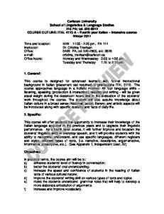
1(0,0) 2(0,7.209) 3(9.391,8.05) 4(-4.919,0.894) 5(7.155,3.578)
s o =4 t o =3 y
t
2
(7)
s
3 1
to 4
(8)
so
2
5 x
1 Figure 1. Reduction of an ellipse
5. THE ALGORITHM
6. CONCLUSION
It is hoped that the reader will forgive, in the interests of brevity and an example of a working program, a coded listing. The seven non-trivial given point coordinates are supplied to produce cos , sin , s0 and t0 . I is the only \tweak" required to resolve the possibility that the sign combination of cos and sin re�ects the desired axis direction about a coordinates axis. The quadratic in cos2 poses an ambiguity in � . Therefore I=-1 will correct an unsuccessful try with I=1. The test example is shown in Fig. 1.
Geometric thinking, a hallmark of engineering design, is exempli�ed by careful choice of initial conditions when formulating a problem, in this case a good coordinate frame. All the theory presented above is pure classical geometry too� largely unknown or forgotten. Anton 2] mentions advanced methods to do the rotation, Lagarange's and Kronecker's reductions, but there is no word of Grassmann. As methods of symbolic computation, which are still quite primitive in this regard, develop, the design engineer will become more a designer of algorithms than a designer of speci�c solutions which will fall into the domain of engineering technicians skilled in the use of advanced software. Similarly, advances in symbolic software will inevitably ressurect the dormant methods of Grassmann and his successors whose results were eclipsed by the \new age" of quantum and relativistic mechanics. These results have lain fallow awaiting application in a future with appropriate computational tools. One may recall that numerical analysis remained an impractical mathematical curiosity until automatic numerical computation established its importance in the '60s and '70s. We toilers in classical mechanics can look forward to the next millenium with great con�dence that new tools will enhance, not eliminate, our jobs, whether in practice or academe.
Programmed Example 100 INPUT Y2,X3,Y3,X4,Y4,X5,Y5,I:Y23=Y2-Y3: Y24=Y2-Y4:Y25=Y2-Y5:REM End of setup 110 Q1=X3*X4*(X4*(Y5-Y3)+X5*(Y3-Y4)+X3 *(Y4-Y5):Q2=X5*(Q1+Y3*Y4*(X3*Y24-X4*Y23)) 120 Q3=Y5*(X4*Y3*(X5*Y23-X3*Y25)+X3*Y4 *(X4*Y25-X5*Y24)):Q=2*Y2*(Q2+Q3) 130 R=Y2*(X4*X5*Y3*Y23*(X4-X5)+X3*(X5*Y4*Y24 *(X5-X3)+X4*Y25*(X3-X4))) 140 P=-2*R:QQ=Q*Q:A=P*P+QQ:B=QQ-2*P*R:C=R*R A2=2*A:IF A=0 THEN STOP 150 D=B*B-4*A*C:IF D