vehicles with a GPS unit and a static GPS database of the road network. With these two, a .... network, and a wireless communication interface (Figure 1). We assume that ...... Verizon Wireless, Inc. http://www.verizonwireless.com. [11] IEEE Std.
Grassroots – A Scalable and Robust Information Architecture Samir Goel1 , Tomasz Imielinski1 , Kaan Ozbay2 , Badri Nath1 {gsamir@cs, imielins@cs, kaan@rci, badri@cs}.rutgers.edu 1
2
Department of Computer Science Rutgers, The State University of NJ Piscataway, NJ 08854
Department of Civil Engineering Rutgers, The State University of NJ Piscataway, NJ 08854
DCS-TR-523 Abstract We propose a novel architecture, Grassroots, for collecting, disseminating, and querying information about the physical world. The Grassroots architecture consists of a massive number of individual agents called dataflies, which move around, collect, summarize, and query information about their immediate physical environments. We make use of this architecture in developing a system for collecting and disseminating real-time traffic information. Such a system would prevent traffic congestion from building up. Today a number of commercial solutions exist for disseminating traffic information (e.g., Traffic.com, Metrocommute, EtakTraffic). However, these solutions are plagued by prohibitive deployment and maintenance cost that prevents widespread deployment. As a result, these solutions cover select highways while leaving out major fractions of the highways. In this paper we present our vision of a low cost, highly scalable zero-infrastructure system for collecting and disseminating information about traffic conditions. Our goal is to devise a system that can cover the entire road network of US. We describe the proposed architecture for the system, and evaluate it using realistic model of transportation network and realistic traffic conditions.
1
Introduction
Imagine a novel location-aware information system where objects such as cars, humans, or cell-phones, equipped with sophisticated sensors, collect information about their physical environment. They either report this information in response to queries or spontaneously disseminate it around. Examples of such data that can be collected include traffic conditions (travel times) as measured by cars, allergen levels (e.g., pollen levels) as measured by sensors on human beings, or signal strength and available bandwidth to indicate spectrum quality and availability as measured by cell phones. Travel times, measured by one car, are of interest to other cars that are likely to take that route. Information about presence of allergic material in a region is of interest to others who are sensitive to the toxins and are intending to pass by that region. Signal quality maps are of interest to the cell phone users who want to know the best locations for making a call. In such a system, each mobile sensor contributes a small piece of information to the ”overall picture”, which is aggregated from multiple such individual reports. We call such an environment Grassroots 1 to signify the ”bottom up” information gathering and dissemination involved. Grassroots consists of a massive number of individual agents, called dataflies, that move around, and collect, summarize, and classify information about 1 Grassroots effort is often used to describe a political campaign that relies on small contributions or large scale individual efforts. This is similar to the way an overall picture of the environment is obtained from data collected from individual mobile data sources.
1
their immediate physical environment. Grassroots is different from the usual sensory environment since it relies on mobile sensors (dataflies) rather than on a fixed predefined infrastructure. Dataflies can visit areas that are not instrumented by sensors. Also, dataflies can offer multiple reports of the same physical space (i.e., cars traveling through the same road segment, or cell phones reporting signal strength in the same area). This highlights two important characteristics of Grassroots environment: redundancy, which imparts robustness, and dynamic nature of coverage, which changes with the location of its dataflies. Grassroots architecture has the potential to create a highly scalable and robust information acquisition system. We believe that transportation is one of the domains that is ideally suited for Grassroots architecture. “Traffic Congestion has become part of daily life in many places as traffic continues to increase on a relatively unchanging highway network. Highway congestion is not just a problem of recurring “rush hour” delay in major cities. More than half of all congestion is non-recurring, caused by crashes, disabled vehicles, adverse weather, work zones, special events and other temporary disruptions to the highway transportation system. Unless we manage highway congestion, our nation will continue to incur economic costs in forgone productivity, wasted fuel, and a reduced quality of life.” [8] According to the Texas Transportation Institute (TTI), the total congestion “bill” for 75 urban areas in the United States in 2000 came to $67.5 billion, which was the value of 3.6 billion hours of delay and 5.7 billion gallons of excess fuel consumed [20]. One possible way of controlling the extent of congestion is by disseminating traffic information. This gives an opportunity to the drivers to bypass congested routes thus preventing congestion from building up. Today a number of commercial systems exist for collecting and disseminating traffic information (e.g., Traffic.com [9], Metrocommute [5], EtakTraffic [4]). However, these systems tend to cover select highways while leaving out a major fraction of roadways, thereby creating a “digital divide”. In case of congestion, if any of alternate routes falls outside the coverage zone, drivers are left to guesswork, past experience, and their instincts in deciding on a faster route to their destination. The main factor that prevents these systems from covering the entire road network of US is the cost involved. Each of these systems requires an infrastructure to be deployed (e.g., helicopters; static cameras at busy intersections and entrances to tunnels/bridges; traffic flow sensors along major highways). This represents a huge amount of money in one-time deployment cost, and a significant recurring cost in maintenance. In order to address the problem of traffic congestion, there is an urgent need for a solution that can be deployed on a large scale at a low cost. In this paper, we present our vision and architecture of a novel information system for collecting and disseminating traffic information that enables all vehicles to be completely aware of the traffic conditions (travel time) relevant to them. We would like the system to be highly scalable, able to cover the entire road network of US. Most importantly, we would like the system to require zero or minimal additional infrastructure. This requirement ensures that cost does not become an issue preventing widespread deployment. We believe that such a system has the best chance of being deployed. Our key idea is to turn vehicles themselves into sensors that collect and disseminate traffic information. This can be done by equipping vehicles with a GPS unit and a static GPS database of the road network. With these two, a vehicle can keep track of its location and determine its travel time for each of the road segment visited. As vehicles travel, they can potentially collect travel time information of the visited road segments. Aggregating and sharing this information with other vehicles would result in an information system where all vehicles are aware of traffic information. Sharing requires communication over wireless link. Since millions of vehicles are involved, if one is not careful, the communication can easily inundate the wireless link. To get an idea of magnitude of the problem, let’s consider a trivial approach to disseminating traffic information. Let’s assume that every vehicle, on traveling a road segment, broadcasts the travel time experienced throughout US2 . All vehicles can locally aggregate the received travel time information to build a complete picture of the traffic information on all road segments in US. Assume that vehicles cover a road segment once every minute, on an average (assume an average vehicle speed of 30 mph and average road segment size of 0.5 mile). It is estimated that there are approximately 100 million vehicles in US. If at maximum half of these were mobile simultaneously, 50 million travel time updates would be generated per minute. This translates into ˜83 Mbps of maximum bandwidth required (assuming that size of each update packet is 100 bits 3 ). 2 Assume 3 Each
for the sake of discussion that there is a mechanism for broadcasting a packet throughout US. travel time update packet would store the id of the road segment, the timestamp, and the travel time information.
2
For comparison note that the capacity of highest speed wireless LAN is 54Mbps (for 802.11a [11]) and the total cell capacity in 2G cellular networks is approximately 600 Kbps (there are typically 60 channels in a cell, each with bandwidth of 9.6Kbps [16]). Clearly, we need some mechanisms for intelligently cutting down the maximum bandwidth required while still meeting the minimum requirements on the “quality of traffic information” available at each vehicle. We make three observations that would help us in cutting down the amount of bandwidth required. Firstly, we observe that one can tolerate degradation in two aspects of the quality of traffic report – delay and accuracy. One can tolerate small amount of delays in the traffic report (e.g., travel time estimate can be 15 mins old). Also, the traffic report need not be exact. One can tolerate small amount of inaccuracy in the travel time estimate (e.g., travel time estimate can be off by 10%). Our second observation relates to the geographic scope of the “view” of the vehicle. We observe that vehicles in CA do not really need to know the current traffic conditions in NJ. This is true for two reasons: Firstly, it is unlikely that vehicles in CA intend to travel to NJ. Secondly, even if some vehicles do intend to travel to NJ, by the time they will get there, the traffic conditions would have changed dramatically. Since traffic information changes drastically in an hour’s time, a vehicle only need to know accurate traffic information of road segments that may be reached in 1 hour (for most of the regions this would translate to a range of less than 80 miles, assuming a maximum average vehicle speed of 80mph). This observation allows us to limit the geographical scope in which traffic information is disseminated, thereby significantly reducing the bandwidth requirement. Thirdly, we observe that the interest (number of queries) in travel time would decrease at a slower rate with distance for highways than that for other types of road segments (e.g., road segments inside a residential complex). Thus, one can cut down the bandwidth requirement by varying the geographic scope in which travel time information for a road segment is disseminated according to its spatial interest gradient. Note that the spatial interest gradient of road segments may change dynamically depending on the time of the day and the current traffic conditions. For example, if a segment of a highway is congested, lot of queries would be directed for road segments on the diversion routes that allow vehicles to avoid the congestion, thus reducing their spatial interest gradient. These will return to normal levels once the congestion clears up. Our goal in this paper is two-fold: (a) identify key performance metrics and key parameters that affect the performance of the system, and (b) examine the effect of various parameters and design choices on the performance of the system. We use Paramics [7], a state-of-the-art micro-traffic simulator, along with a calibrated model of Southern New Jersey transportation network for this purpose. We identify the research issues that need to be resolved before a practical system can be built. In the next section, we survey the related work in this area. In section 3 we give an overview of the system. In section4, we describe the proposed architecture for the system. In section 5 we enumerate the performance metrics. In section 7 we detail the mechanisms involved. In section 8, we evaluate the proposed mechanisms. In section 11 we outline our future work.
2
Related Work
At the architectural level, Data Mules project[21] is closely related to the proposed Grassroots architecture. In Data Mules project, authors propose to use a set of mobile agents for supporting communication among a set of sparsely distributed sensors. Grassroots architecture goes beyond Data Mules idea in that not only the communication layer but also the sensing components are mobile. As discussed earlier, this results in two key characteristics to the system: firstly, with mobile sensors, one can cover wider area with fewer sensors, and secondly, the inherent redundancy in the system imparts robustness to the system. Recent parallel projects [22, 23, 15, 18] have also proposed using vehicles as sensors of traffic information. In [15] authors propose using AVL-equipped transit vehicles as probe vehicles for estimating traffic information. In TRANSMIT [18] authors use Electronic Toll and Traffic Management (ETTM) equipment, We expect road segment id would take 32 bits (100 million road segments), timestamp would take 32 bits, and travel time information would take 16 bits, with some bits for header.
3
compatible with E-ZPass System4 for traffic surveillance and incident detection. These projects, and the work by Brackstone et al [12], Chen et al [13], and Elango et al [17] demonstrate that it is feasible to use vehicles as traffic information sensors. Our work can be seen as extending these in two important ways: firstly, we attempt to use potentially every vehicle as a traffic sensor. We expect this to result in wider and better coverage (section 3). Secondly, we attempt to do away with the requirement of any centralized system and infrastructure (e.g., toll booths). In [22, 23] authors propose equipping vehicles with short-range wireless link (e.g., IEEE 802.11 [11]) for spreading traffic information. Wischhof et al [22] suggest having each vehicle periodically transmit its position, velocity, and heading, along with aggregate traffic information5 . Ziliaskopoulos et al [23] suggest having vehicles exchange recent travel time information with vehicles traveling in the opposite direction. As discussed in section 3 and 7.1, in order for the traffic information to be useful, drivers need to know it well in advance (a few miles, in some cases) to be able to avoid congested routes. With short-range wireless link, propagating traffic information a few miles would require many vehicle-to-vehicle communication hops, and would be feasible only in regions with sufficiently high vehicle density. This may not be true for all the regions (rural regions have low vehicle density) and at all times (vehicle density decreases substantially in the night). The proposed solutions cannot be carried over to wide-area wireless link (e.g., cellular network) where bandwidth is precious and expensive. In our work, we propose using wide-area wireless link and our emphasis is on controlling the bandwidth consumption while retaining requisite level of awareness of traffic conditions among vehicles.
3
System Overview
The design space for systems that can collect and disseminate traffic information is large. We envision a highly scalable system that exploit existing infrastructure and require minimal or zero additional infrastructure. Systems based on such designs will arguably have low deployment and maintenance cost. We believe such systems have the best chance of being deployed on a large scale. We envision that every participating vehicle would be equipped with a device that we call TrafficRep. This device is responsible for collecting and disseminating traffic information (we describe it in more detail in section 3.1). The TrafficRep device connects to the in-vehicle navigation system (e.g., 750NAV from Magellan [1]), supplying it with current traffic conditions. From a user’s (driver) perspective, TrafficRep device appears as a black box. A user only interacts with the in-vehicle navigation system posing queries like, “What is the fastest route from Busch Campus to Newark Airport?” The in-vehicle navigation system, in turn, queries the TrafficRep device to obtain current traffic information on various road segments, computes the fastest route, and displays it to the user. Figure 1 shows the schematic diagram for the system. In response to a query, the TrafficRep device may either respond with the information that it already has, or it may pose the query to TrafficRep devices located in other vehicles. The driver has no direct control over this decision. This prevents a user from intentionally/unintentionally flooding the wireless channel with queries. Assuming that “enough” vehicles in an area have TrafficRep device on them, these vehicles collectively store to-the-minute traffic information for the area. However traffic information of interest to a vehicle is potentially distributed across a number of highly mobile vehicles. In order to achieve the goal of traffic awareness, the system needs to support three basic operations in order to get the data from vehicles having desired traffic information to vehicles requesting traffic information: • Querying: This operation allows a vehicle to query the traffic conditions on a road segment. Note that vehicles would typically issue a query for traffic conditions on a stretch of route. Such a query can be thought of as issuing multiple queries, one for each road segment on the queried route. • Monitoring: This operation allows a vehicle to monitor the traffic conditions on a road segment. Whenever the travel time on a road segment changes appreciably, the vehicle receives an update. 4 E-ZPass
is an electronic toll collection system, currently in operation in NY/NJ/CT metropolitan areas traffic information is computed based on periodic reports received by the vehicle
5 Aggregated
4
GPS
Static GPS database of road network
Wireless Interface
Database of current traffic conditions
TrafficRep Device Query for traffic conditions Query for route DRIVER Response
Response
In−vehicle navigation system
Figure 1: Schematic diagram of the components that will be present in each participating vehicle in the envisioned system • Dissemination: This operation entails broadcasting/multicasting traffic information in a specified geographic area. For frequently requested traffic information, it may be more bandwidth efficient to disseminate the information proactively. The important features of this system are: 1. The system consists of millions of highly mobile sensor nodes (TrafficRep devices on vehicles 6 ). This has two consequences: • The coverage provided by the vehicles is dynamic and changes with the location of vehicles. • Multiple vehicles may sense the travel time of each road segment at around the same time, introducing redundancy in information collected by the vehicles. This redundancy is critical to the resilience and reliability of the system. 2. Turning vehicles into traffic sensors has the advantage that zero additional infrastructure is required. However the disadvantage is that awareness of traffic information on a road segment is available only if there is relatively uniform flow of vehicles through that segment. If there are no “witnesses” even temporarily, that information is not available. The only exception to this limitation is when “enough” fraction of vehicles are instrumented. Then “no news is good news” – if there are no witnesses to traffic on a given road segment it means that there is no traffic. 3. For traffic information to be useful, a vehicle should receive it well in advance to be able to take an alternate faster route. This is especially true for highways, where the diversions points (exits) are typically separated by a “few”miles. This suggests that a typical querying, monitoring, or dissemination operation would involve communicating travel time information over a relatively long distance (“few” miles). 4. Density of participating vehicles in an area may vary dramatically with time (usually it drops substantially at night) and space (rural regions typically have lower vehicle density than urban ones). 6 Many times in this paper we use vehicles to refer to “TrafficCom device in the vehicle”. The intended meaning should be clear from the context.
5
The fact that traffic information is needed well in advance coupled with the fact that density of vehicles may vary dramatically with space and time, have direct implications on the type of wireless links that may be used with the TrafficRep device. We discuss this in more detail in section 7.1.
3.1
TrafficRep device
A TrafficRep device is attached to three components: a GPS device, a static GPS database of the road network, and a wireless communication interface (Figure 1). We assume that the static GPS database is organized by road segments, where a road segment is a stretch of a road between two successive exit points (junction, exits, etc). It is estimated that there are about 7 million road segments in US. For each road segment, the database stores three attributes: 1. GPS coordinates of its endpoints, 2. Length of the segment, and 3. Free flow traveling time (length of the segment divided by the free-flow speed limit). TrafficRep uses the location and time information from the GPS unit and the static information about location of end-points of road-segments to calculate the travel time of vehicle for different road segments. Every time the vehicle travels on a road segment, TrafficRep records the corresponding travel time information as a travel log report (TLR). This includes identifier of the road segment, the travel time, and the time-stamp of the report. As TLRs get older, they are discarded by the TrafficRep device to create space for new ones. The wireless communication interface may be a short-range communication link (e.g., 802.11 flavor) or a wide-area communication link (using cellular network [6] or two-way paging network). Our only requirement from the wireless communication interface is the capability to perform broadcast or multicast. We discuss the pros and cons of different type of links in section 7.1. TrafficRep device uses the wireless communication interface in order to support the basic operations: querying, monitoring, and dissemination. The requirement that every vehicle be equipped with TrafficRep device along with GPS device and invehicle navigation system may seem like a deviation from our goal of zero additional infrastructure design. There are two important reasons for this requirement: Firstly, we expect vehicles in future to come equipped with GPS device and in-vehicle navigation system. These two components have already started to appear even in low-end vehicles. Also, we expect TrafficRep device in itself to be quite cheap. This plus the fact that users may be willing to bear a part of its cost makes the deployment cost very small compared to that of existing solutions, for the same coverage. Secondly, equipping each vehicle with a device naturally makes the owner responsible for it. Thus, the cost of maintaining the system would be very small compared to that for equipment (cameras, helicopters, etc) needed in existing commercial solutions.
4
Proposed Architecture
The Grassroots architecture has four entities: information producers, information consumers, information aggregators, and information relayers. Producers are vehicles (dataflies) that collect raw sensory data. Consumers are objects (stationary or mobile) that query data (e.g., vehicles). Aggregators collect and aggregate data from multiple producers. An aggregator is a logical entity that can reside on a stand-alone server or can even reside on a consumer. Relayers participate in forwarding messages to their intended destination. In the transportation domain, with potentially millions of vehicles involved, the primary challenge in disseminating and querying dynamic sensory information is scalability. Both high scalability as well as zero additional infrastructure requirements makes peer-to-peer a natural architecture to investigate for us. In this architecture, vehicles communicate directly with other vehicles to disseminate traffic information and to process queries. This is in contrast to the centralized architecture, where all vehicles report traffic information to a central server, and the central server disseminates traffic information and answers queries 6
from the vehicles. The centralized solution has three serious drawbacks: Firstly, the central server is single point of failure. Secondly, the central server may become a bottleneck for a system with millions of vehicles querying and updating it. Finally, having a central server brings in deployment and maintenance costs. We still simulate centralized solution in order to use its performance as a benchmark against which we compare the performance of our peer-to-peer solution.
5
Performance Metrics
In the proposed peer-to-peer architecture, vehicles communicate directly with other vehicles. In section 1, we estimated that it would require ˜83 Mbps bandwidth for the extreme case where every vehicle broadcast the collected TLR throughout US, every time it finishes traveling a road segment. Clearly it would not be possible to support this huge bandwidth requirement using the existing communication infrastructure. The important question is how to cut down on the bandwidth required while still maintaining a requisite level of accuracy in the knowledge of traffic conditions among vehicles. This suggests four performance metrics: 1. Awareness: This defines the minimum quality of monitoring possible in the system. For example, a vehicle is said to be aware of the query, “What is the travel time on NJTP between exit 9 and 10? ”, with an error margin of 5%, if its knowledge of travel time is always within 5% of the true value. 2. Observability: This defines the minimum quality with which the system answers a query. For example, the system is said to be observable for the query, “What is the travel time on NJTP between exit 9 and 10?”, with an error margin of 5%, if it can provide answer that is always within 5% of the true value. 3. Coverage: This is expressed in terms of the fraction of road network for which the system can support requisite level of observability and awareness. 4. Wireless bandwidth used: It is important to keep the wireless bandwidth usage low. This is especially important when using commercial wide-area wireless link like cellular network, as every transmission has a cost associated with it. As a result the number of messages transmitted directly affects the cost of operation of the system. It is important to decide on a measure of awareness carefully. For a better understanding, consider the question: Is the awareness low if a vehicle in California is not know the traffic conditions in NJ? More generally, does the awareness decrease if a vehicle does not know the travel time on a road segment that it is not intending to take? An indirect way of measuring the performance of the system is to consider the vehicles’ travel time, and how close it is to the ideal one where the vehicle has complete traffic information. After all travel time is the metric that most users are directly concerned with. A more detailed study of other relevant performance metrics is a subject of our future work.
6
Scope of the paper
As our first step, we assume that the system only provide support for dissemination mechanism. This simple setup allows us to investigate the effect of key parameters affecting performance. In this system a TrafficRep device maintains an estimate of the travel time on all the links. In the absence of any additional information, this estimate is set to the free-flow travel time on the link (obtained from static database of the road network). On receiving disseminated traffic reports, the vehicles update their travel time estimates. Since querying operation is not supported, the TrafficRep device assumes that the traffic information available locally is the accurate information. We investigate different dissemination mechanisms that would keep this local information close to the true value, and examine the bandwidth-usage versus accuracy tradeoff. Support for querying and monitoring operation is a subject of our future work.
7
function naive scheme() L : set of recently visited links Lrep : set of links that the vehicle has already disseminated information about ˆ expected travel time for link l e(l): e(l): travel time actually experienced by the vehicle for link l tlast : time of last dissemination for this vehicle tcur : current time λ: maximum rate of dissemination if (tcur − tlast > λ)
ˆ ); lmax = arg maxl∈L−Lrep ( e(l) − e(l) disseminate link info(lmax ); end
Figure 2: Pseudo-code for Naive scheme
7
Dissemination Mechanism
In order to disseminate information about traffic conditions, a vehicle needs to take three decisions: when to send the TLR, what to include in the TLR, and where to disseminate it. These three decisions are interrelated and they determine the bandwidth requirement of the system. In this paper, we explore two schemes for deciding what and when to disseminate: 1. Naive Scheme: Vehicles have a pre-defined maximum rate of dissemination. In this scheme, the vehicles transmit a TLR periodically, at the maximum rate of dissemination. Whenever it is time to transmit a TLR, the vehicles looks at the set of recently traveled road segments and selects the one for which the expected travel time differed the most from the travel time actually experienced by this vehicle. The pseudo-code for this scheme appears in figure 2. 2. Smart Scheme: In this scheme, vehicles send a TLR only when they have something “interesting” to report. Here, vehicles have a pre-defined maximum rate of dissemination. Also, periodically every vehicle selects the most promising road segment to report about. However, unlike in Naive scheme, a vehicle goes ahead with the transmission only when the expected travel time on the road segment (known to the vehicle prior to traveling on this road segment) differs significantly from the travel time experienced by the vehicle. The pseudo-code for this scheme appears in figure 3. In both the solutions, vehicles always disseminate traffic report about a road segment R in a geographic area centered on R. The size of the geographic area is determined by the dissemination scope. In our evaluation, we have chosen to keep the scope of dissemination as a parameter and evaluate the performance for different scope. In general, we would expect that larger the scope, the higher the chances that vehicles would know of traffic congestion and would be able to find a faster alternative route. The flip side is that the larger the scope, the more the number of broadcasts, resulting in higher bandwidth usage. This may translate into higher cost in case the link is a commercial wide-area wireless link (section 7.1). We compare the performance of the proposed mechanisms based on peer-to-peer architecture with that for mechanisms based on centralized architecture. In the centralized solution, vehicles send their TLRs to the central server. They use the above two schemes, Naive and Smart, in order to decide when and what to report to the central server. The central server also needs to take decision on what, when, and where to disseminate. We discuss this in more detail in section 7.3.
7.1
Wireless link
We now examine the suitability of short-range and wide-area wireless link to the solution. Solutions relying only on short range communication link (e.g., 802.11 flavor) for propagating traffic information hop-by-hop 8
function smart scheme() L : set of recently visited links Lrep : set of links that the vehicle has already disseminated information about ˆ expected travel time for link l e(l): e(l): travel time actually experienced by the vehicle for link l tlast : time of last dissemination for this vehicle tcur : current time λ: maximum rate of dissemination ∆: minimum change threshold ff(l): travel time for link l based on its speed-limit (free-flow) h(l): last travel time report heard link for l. Reports heard more than k secs ago are discarded disseminate = true; if (tcur − tlast < λ) return; end
S = {∀l ∈ L − Lrep | h(l) = null ∨ |h(l) − e(l)| > ∆};
← Among the links which were never reported, exclude the ones for which the travel time recently heard is “quite” similar to what was experienced
ˆ ); lmax = arg maxl∈S ( e(l) − e(l)
ˆ if ( e(lmax ) − e(lmax ) < ∆)
← check if the information is “interesting”
if (|ff(lmax ) − e(lmax )| < ∆) disseminate = false; end end if (disseminate) disseminate link info(lmax ); end
← check if travel time differs significantly from free flow
Figure 3: Pseudo-code for Smart scheme
9
have limited feasibility because of the number of hops involved in communicating information over such large distances. These would be feasible only in regions where the density of participating vehicles is high. Any “hole” along the route would stop the propagation of information, especially if the information being propagated is upstream with respect to flow of traffic. Since the density of vehicles vary considerably over a day, even in regions with high traffic density during peak hours, the feasibility of propagating information over long distances may diminish during off-peak hours. We investigate the use of wide-area wireless link (e.g., two-way paging network, cellular network) in our system. Their “near-universal” presence makes them an ideal candidate for the proposed system. We assume that the wide-area wireless network allows a vehicle to broadcast a message in the local cell (e.g., for cellular network this may entail sending a text message (SMS) to a specific cell-broadcast address). Note that this capability is already present in exiting cellular systems [16], though a normal user is not allowed to use it7 . However, allowing vehicles to perform a local cell broadcast would enable them to disseminate a TLR in a few square miles area with a single transmission (cell size in a cellular network is typically between 1Km to 35 Kms [16]). Unlike an 802.11 link, every transmission using the cellular network has a cost associated with it. As a result, the number of transmissions in the system contribute to the recurring operational cost of the system. This cost will ultimately get passed down to the individual customers. In order for the system to be practical it is crucial that vehicles achieves requisite awareness with as few transmissions as possible. The investigation of a hybrid solution that makes use of both short-range but free communication and wide-area wireless link to achieve better cost versus awareness tradeoff is a subject of our future work. As stated earlier, disseminating traffic information of general interest would reduce the number of queries. Here, a vehicle disseminates a TLR directly to other vehicles using cell broadcast. We associate a geographic scope with each TLR. We express this scope in terms of TTL8 . The TTL is expressed in terms of the number of hops of the cells in the cellular service. We make the simplifying assumption that the concept of TTL is supported by cellular network. With this assumption information relayers are not needed in the system. Investigation of how vehicles can collaborate and communicate to implement the concept of TTL is part of our future work. We discuss this in section 10.
7.2
Peer-to-peer solution
In the vehicle-to-vehicle solution, the TLR collected by a vehicle (information producer in this case) is sent directly to other vehicles via a wireless link. Aggregation of information is performed on the receiving vehicle – the information consumer. Each vehicle maintains an estimate of the travel time on all the road segments. On receiving a TLR, the vehicle updates its estimate of the travel time according to equation 1. ˆ = αe(l) ˆ + (1 − α)travel-time e(l)
(1)
ˆ refers to the estimate of the travel time for link l, α represents the decay factor, and travel-time where, e(l) refers to the travel time reported in TLR for link l. Each TLR is disseminated in a geographic scope determined by its associated TTL. Consequently, each vehicle is aware of all information produced in the dissemination scope and can locally answer all queries with scope less than the dissemination scope.
7.3
Centralized solution
We simulate centralized solution in order to use its performance as a benchmark against which we compare the solutions of proposed schemes. In this solution, vehicles send TLR directly to the central server. Server maintains an estimate of travel time on all the road segments. Every time it receives a TLR containing a recent travel time experienced by a vehicle on a road segment, it updates this estimate (using equation 1). 7 Only content providers (providing news, weather information, stock quotes) with tie-ups with cellular service providers are currently allowed to use the local broadcast feature [2]. 8 This is analogous to the concept of time-to-live (TTL) in wired networks.
10
function server decide link() L : set of all road segments links ˆ current expected travel time for link l e(l): ∆: minimum change threshold τ : minimum time interval between successive reports about the same link ff(l): travel time for link l based on its speed-limit (free-flow) rep(l): last travel time reported for link l tlast (l): time at which travel time for link l was last sent tcur : current time
ˆ ) lmax = arg maxl∈L ( rep(l) − e(l)
ˆ ) ≥ 4) if ( rep(lmax ) − e(lmax
← check if the information has changed since the last report
return lmax else ˆ ) lmax = arg maxl∈L ( ff(l) − e(l) // check if the information is “interesting” and last report about this link was sent “some” time ago
ˆ ) ≥ 4) ∧ (tcur − tlast (lmax ) > τ ) if ( ff(lmax ) − e(lmax return lmax end end return φ ← return null
Figure 4: Pseudo-code that a central server uses in deciding the link whose travel time is disseminated Also, if the server does not receive any TLR for a road segment for Tage for units of time, it resets its estimate to the free-flow travel time on the link. Central server continuously checks if it has any “interesting” traffic information to disseminate. For dissemination, it selects the link for which its estimate of travel time differs the most from what it disseminated last, and this difference is greater than a certain minimum threshold. The pseudo-code for the procedure appears in figure 4. When vehicles receive a traffic report from the central server, they simply set their estimate to the one reported.
8
Simulation
In order to evaluate the effectiveness of the two schemes, we have simulated a number of scenarios for disseminating travel time information for various road segments. Indeed, awareness of the travel time is very important especially pertaining to road segments relevant to the travel plan of a vehicle. This information, when up to date, allows a vehicle to avoid congested routes. We have performed extensive simulations using the Paramics simulator [7] to demonstrate the effectiveness of the proposed schemes for disseminating travel time information. Paramics simulates vehicular traffic, down to the level of behavior of each individual vehicle. It incorporates models for controlling microscopic behaviors such as propensity for lane change, gap between vehicles, aggressiveness of drivers, etc. Through its API, Paramics allow a programmer to maintain state on a per vehicle basis and alter the behavior of vehicles programmatically, including the path being followed by it. We extended the set of available APIs in two important ways: • We added features for simulations vehicles that take fastest route using Dijkstra’s shortest path algorithm [14]. • We added features for simulating cellular infrastructure that is geographically overlaid on the simulated road network. We divide the region encompassing the simulated road network into rectangular cells, and simulate a base station in each cell. Cars use cell-broadcast primitive to disseminate travel time information. 11
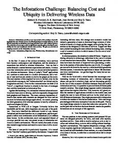
(a) Snapshot
(b) Incident site
Figure 5: Snapshot and incident site To be meaningful, it is important to evaluate the performance of the proposed schemes using realistic data. To this end, we have chosen to simulate the peak afternoon traffic in Southern New Jersey area. Figure 5(a) shows the snapshot of the simulated transportation network. The transportation network model [19] used includes most of the highways in Southern New Jersey. The transportation network model consists of approximately 4000 road segments drawn to closely match reality. Highways drawn match the ones in reality in the number of lanes, length, and posted speed limits. The parameters controlling the flow in our simulations were based on the data provided by the Delaware Valley Regional Planning Commission (DVRPC [3]) and calibrated in [19] to make sure that the traffic characteristics closely match the ones seen in reality.
8.1
Simulation Methodology
In Paramics, the transportation network consists of zones that serve as entry and exit points for vehicles. In order to simplify our analysis we consider only the vehicles traveling between a specific origin-destination zone pair. We believe that the results would hold qualitatively for all origin-destination (OD) zone pairs. Although all participating vehicles are involved in information dissemination, only the vehicles traveling between the target OD pair make use the traffic information gathered in determining the fastest path to the destination. We classify the vehicles traveling between the target OD pair into two categories based on the routes they follow: default and fastest. The default vehicles always follow the fastest route based on the free-flow travel times in the network. This route is computed a priori and it does not change during the entire simulation. For all the simulations this default route remains the same. The fastest vehicles keep recomputing the fastest route to the destination based on the travel-log reports received. They alter their routes if an alternate route allows them to get to their destination faster. Only a fraction of the vehicles traveling between the target OD pair are categorized as fastest. This is to decouple the navigation problem that would arise from having all the vehicles choose the fastest route to the destination. In order to concentrate solely on the problem of effective dissemination of traffic information, we inject fastest vehicles at regular intervals into the network. These serve as probes in the network, continuously testing the accuracy of disseminated traffic information. The interval is chosen so as to keep the number of fastest vehicles small enough that they do not affect the travel time experienced by default vehicles, but large enough to continuously test the effectiveness of dissemination mechanism. 12
Parameter Incident Location Incident Start Time Incident Duration
Value On the exit ramp from HWY I-76 (fig 5(b)) 40 mins 25 mins
Table 1: Parameters controlling the simulated incident We measure awareness indirectly using total travel time. Total travel time for a class of vehicle is the sum of the travel time of all the vehicles of the same class traveling between target OD pair. Clearly, vehicles with accurate travel time information will experience smaller travel time. Thus this metric captures the effectiveness of the dissemination algorithm. In order to evaluate the effectiveness of the dissemination mechanism, we simulate an incident on the default route in our simulations. This incident results in closure of lanes. The parameters of the incident are listed in Table 1. The incident site is shown in the zoomed-in section of the transportation network in figure 5(b). We use the following parameters to control the behavior of the dissemination algorithms: 1. Maximum rate of dissemination: Vehicles in the simulation are not allowed to disseminate faster than a certain pre-defined maximum dissemination rate. The actual rate of dissemination is dependent on the specific mechanism used. The different values of maximum dissemination rate used in the simulations are: once every 60 secs, once every 300 secs, and once every 600 secs. 2. Geographic scope of each TLR: In our simulations, we divide the physical region in rectangular cells of size 2 Km x 2Km. Cells of this size would come under the “small” category in a real cellular network (cell sizes typically vary in radius from 1Km to 35 Kms [16]). We chose smaller size in order to examine, at a finer level, how far the information needs to be propagated for it to positively affect travel time of vehicles. We express geographic scope in terms of TTL, which controls the number of hops a TLR travels. The TTL values used in the simulation are: 1, 2, 3, and 5 (dissemination scope of TTL=5, centered at the accident site, covers the entire simulated road network). 3. Dissemination scheme: We evaluate the performance of Naive scheme and Smart scheme for dissemination. 4. Market Penetration: This determines the percentage of vehicles participating in the dissemination mechanism. Clearly, the percentage of participating vehicles determines the effectiveness of coverage. In order for the system to be effective the market penetration should be above a certain threshold. We vary the market penetration to explore its effect on performance.
8.2
Simulation Results
We start by examining the effect of above parameters on the performance of peer-to-peer scheme. The impact of these parameters remains the same, qualitatively for the centralized scheme. We then compare the performance of centralized scheme with peer-to-peer scheme. 8.2.1
Peer-to-peer solution
Effect of TTL We examine the effect of TTL on the performance of Naive dissemination scheme. The maximum dissemination rate is set to once per 60 secs, and we simulate a market penetration of 10%. Figure 6 summarizes the result. The bar graph plots for different values of TTL, the percentage reduction in the travel time of fastest
13
% Improvement in Average Travel time versus TTL [Max dissemination rate: 60 secs, Scheme: Naive, Market Penetration: 10%] 25
% Improvement in Avg Travel time over Default
20
15
10
5
0
−5
1
2
3 TTL
5
Figure 6: Summary of the performance of Naive scheme for different values of TTL vehicles over that of default vehicles during the accident period9 . As expected the performance improves with increase in TTL. For TTL=1, the performance of fastest vehicles is very similar (slightly degraded) to that of default vehicles. This is to be expected because by the time the vehicles come to know of the higher trip times on road segments they are too close to the traffic congestion and do not have any better alternative route to avoid it. With larger value of TTL, the vehicles get know of congestion state in advance and are able to avoid it by taking an alternative faster route. This clearly illustrates the importance of disseminating traffic information in a wider geographic scope. Note that the amount of improvement achieved is also a function of the duration of incident and the number of lanes affected by it. Clearly if an incident lasts longer and affects more lanes, potentially fastest vehicles will see greater reduction in travel time over default vehicles. Effect of maximum rate of dissemination We investigate the effect of the maximum rate of dissemination on performance. Consider a road segment, R. As stated earlier, the dissemination scope of every TLR reporting travel time on R has an associated geographic scope centered on R. For a fixed TTL, the geographic region in which TLRs for reports about R are disseminated remains constant. Vehicles outside the dissemination scope have very little idea about the traffic conditions on R. When a vehicle enters the dissemination scope for R and is intending to travel on this road segment, there is a limited window of time in which it should be warned about any congestion on R. As the vehicle gets closer to R, it has fewer alternate (faster) routes that avoid R. The rate of dissemination should be chosen such that with a very high probability, the vehicle hears at least one congestion report while it still has an option of avoiding it. The required rate of dissemination is directly proportional to the length of window of time available to vehicles. This would argue for a very high dissemination rate. However, the flip side is that higher the dissemination rate, the more the number of messages transmitted, resulting in higher cost of operation. In order to illustrate the impact of maximum dissemination rate, we performed simulation with TTL value of 3, market penetration of 10%, and with Naive dissemination scheme. Figure 7(a) shows the impact of change in maximum dissemination rate on the performance (the percentage improvement in travel time of fastest vehicles over default vehicles). TTL value was set to 3 because for this setup it gives close to peak performance (figure 6). This helps us in isolating the impact of maximum dissemination rate. As the scope increases, the window of time available to a vehicle to choose an alternate route increases. This implies that increase in TTL can compensate for decrease in rate of dissemination. The performance graph for TTL=5 shown in figure 7(b) illustrates this. 9 The
summary graph shows data points that are average over three runs.
14
% Improvement in Average Travel time versus Max dissemination rate [TTL: 3, Scheme: Naive, Market Penetration: 10%]
% Improvement in Average Travel time versus Max dissemination rate [TTL: 5, Scheme: Naive, Market Penetration: 10%]
25
30
% Improvement in Avg Travel time over Default
% Improvement in Avg Travel time over Default
25 20
15
10
5
20
15
10
5
0
60
300 Max dissemination rate (secs)
0
600
(a) TTL=3
60
300 Max dissemination rate (secs)
600
(b) TTL=5
Figure 7: Simulation results showing the effect of max rate of dissemination on the performance
Naive versus Smart scheme With respect to the number of messages transmitted the Smart scheme outperforms Naive scheme by a wide margin, an order an magnitude in certain cases. Figure 8(a) shows the average number of messages transmitted per cell for different values of TTL, for 10% market penetration and maximum dissemination rate of 60 secs. Figure 8(b) shows the average number of messages transmitted per cell for different values of maximum rate of dissemination for TTL of 3. These results are to be expected because in Smart scheme vehicles transmit a message only when they have something “interesting” to communicate. Now consider the effect on travel time. Figure 9(a) compares the travel time for the two schemes for different values of TTL for the case when the maximum rate of dissemination is 60 secs and the market penetration is 10%. Figure 9(b) compares the performance of two schemes for different maximum dissemination rates. Somewhat counter-intuitively Smart scheme performs better with respect to travel time. This is because in Smart scheme vehicles transmit only “interesting” travel time information. As a result, the travel time estimates of vehicles are able to follow the true travel time more closely. This is especially true for road segments whose travel time information is changing quickly. Effect of market penetration The higher the market penetration, the closer we get to the ideal case where for every road segment there are always vehicles sensing traffic conditions on it and reporting if they detect anything unusual. Intuitively this should transform into greater improvement in travel time of the vehicles. We examined the performance for three different values of market penetration: 5%, 10%, and 20%. We considered two cases. In the first case, we kept the maximum dissemination rate constant at 60 secs and varied the scope of dissemination (TTL). In the second case, we kept the TTL fixed at 3 and varied the maximum dissemination rate. Results for the two cases appear in figure 10. For both the cases we see that the performance improves as the market penetration increases. Smart scheme performs slightly better than Naive scheme because vehicles’ travel time estimate is able to follow the change in true travel time very closely. We find that for Smart Scheme, graph for number of messages increases versus market penetration increases in the beginning, but flattens out for higher values of market penetrations. This is to be expected
15
Avg number of messages transmitted per cell versus TTL [Max dissemination rate: 60 secs, Market Penetration: 10%]
4
2.5
x 10
Avg number of messages transmitted per cell versus Max dissemination rate [TTL: 3, Market Penetration: 10%] 9000
Naive Smart
Naive Smart
2 Avg number of messages transmitted per cell
Avg number of messages transmitted per cell
8000
1.5
1
0.5
7000
6000
5000
4000
3000
2000
1000
0
2
3 TTL
0
5
60
(a) Maximum rate of dissemination: 60 secs
300 Max dissemination rate (secs)
600
(b) TTL=3
Figure 8: Simulations results comparing the number of messages transmitted per cell for Naive and Smart scheme (market penetration: 10%)
% Improvement in Average Travel time versus Max dissemination rate [TTL: 3, Market Penetration: 10%]
% Improvement in Average Travel time versus TTL [Max dissemination rate: 60 secs, Market Penetration: 10%] 30
25 Naive Smart
Naive Smart
% Improvement in Avg Travel time over Default
% Improvement in Avg Travel time over Default
25
20
15
10
20
15
10
5
5
0
2
3 TTL
0
5
(a) Maximum dissemination rate = 60 secs
60
300 Max dissemination rate (secs)
600
(b) TTL=3
Figure 9: Simulation results comparing the performance of Naive and Smart scheme with respect to improvement in travel time
16
% Imporvement in Avg Travel time versus Market Penetration [Scheme: Smart, Max Dissemination Rate: 60 secs] 30
Max Rate: 60 secs Max Rate: 300 secs Max Rate: 600 secs % Improvement in Avg Travel time over Default
% Improvement in Avg Travel time over Default
25
20
15
10
25
20
15
10
5
5
0
% Improvement in Avg Travel time versus Market Penetration [Scheme: Smart, TTL: 3]
30
TTL: 2 TTL: 3 TTL: 5
0
5%
10% Market Penetration (%)
20%
5%
10%
20%
Market Penetration (%)
(a) Maximum dissemination rate = 60 secs
(b) TTL = 3
Figure 10: Effect of market penetration on performance of Smart scheme because in Smart scheme vehicles only transmit “interesting” information (we omitted this graph for lack of space). 8.2.2
Centralized solution
In this section, we compare the results for peer-to-peer and centralized solution (in both cases, Smart scheme is used). When compared in terms of improvement in travel time, the two schemes have similar performance (figure 11) with peer-to-peer solution performing slightly better in some cases. However, when compared on the basis on number of messages received per hour, centralized scheme performance much better than the peer-to-peer scheme (figure 12). The reason is that in centralized solution the central server makes more efficient use of down-link bandwidth. Peer-to-peer solution does not fare well because vehicles take independent decisions on when to transmit a TLR. In our ongoing work, our goal is to bring the bandwidth usage of peer-to-peer solution as close to the centralized solution as possible.
9
Discussion
For cellular networks, since every transmission has a cost associated with it, operational cost may be one of the relevant performance metrics. For any system, the operational cost of the system gets distributed over the number of subscribers in the system. In our zero-infrastructure solution, the only operational cost is the carrier charge for the number of messages transmitted. In order to be able to translate from the number of messages transmitted to corresponding dollar amount, we perform back-of-the-envelope calculations based on the current rate charged by wireless carriers for sending/receiving a SMS message and some simplifying assumptions. The current rate charged by wireless carriers for sending or receiving a message is approximately 1 cents [10]. With this rate the total cost involved in sending a message from one mobile to another is 2 cents. We make the simplifying assumption that senders will be charge 2 cents/message for sending a broadcast message in a cell (because of the difficulty in keeping track of identity of cell phones that received the message). In figure 13 we translate the number of messages transmitted and received per hour for peer-topeer and centralized scheme into cost per subscriber per month. Since we are simulating peak hour traffic, we translate the per hour number into per day figure by assuming that the number of messages communicated 17
% Improvement in Average Travel time versus TTL [Max Dissemination Rate: 60 secs, Market Penetration: 20%]
% Improvement in Average Travel time versus Max dissemination rate [TTL: 3, Market Penetration: 20%]
30
30 Client−Server Peer−to−Peer
Client−Server Peer−to−Peer
25 % Improvement in Avg Travel time over Default
% Improvement in Avg Travel time over Default
25
20
15
10
5
20
15
10
5
0
2
3
0
5
60
300 Max dissemination rate (secs)
TTL
(a) Max dissemination rate: 60 secs
600
(b) TTL = 3
Figure 11: Simulation results comparing the performance of peer-to-peer and centralized solution for two cases: (a) maximum dissemination frequency is kept constant at 60 secs, (b) TTL is kept constant at 3
# of Messages received/hour versus Max dissemination rate [TTL: 3, Market Penetration: 20%]
# of Messages received/hour versus TTL [Max dissemination rate: 60 secs, Market Penetration: 20%]
700 Client−Server Peer−to−Peer
Client−Server Peer−to−Peer
600
2000
# of Messages received/hour
# of Messages received/hour
500 1500
1000
400
300
200 500
100
0
2
3
0
5
60
300
600
Max dissemination rate (secs)
TTL
(a) Max dissemination rate: 60 secs
(b) TTL: 3
Figure 12: Simulation results comparing the performance of peer-to-peer and centralized solution on the basis of number of messages received/hour
18
per subscriber cost/month versus Max dissemination rate [TTL: 3, Market Penetration: 20%]
per subscriber cost/month versus TTL [Max dissemination rate: 60 secs, Market Penetration: 20%]
25 Client−Server Peer−to−Peer
Client−Server Peer−to−Peer
70
20 per subscriber cost/month (dollars)
per subscriber cost/month (dollars)
60
50
40
30
15
10
20
5 10
0
0 2
3
5
60
300
600
Max dissemination rate (secs)
TTL
(a) Max dissemination rate = 60 secs
(b) TTL = 3
Figure 13: Estimate of per subscriber cost per month for peer-to-peer and centralized solution (market penetration: 20%) per day would be approximately seven times (according to [20] average duration of congestion per day across 75 urban areas in US is seven hours). We use this to obtain an estimate for number of messages per month. We divide this operational cost to the number of participating vehicles in the simulation to get the per subscriber charge per month. It shows that even with very simple schemes, we get very close to the $10.0 mark charged by some traffic information systems (e.g., Traffic.com [9] charges $9.95 per month for 40 queries from its subscribers).
10
Future Work
There are a number of research issues that remain to be resolved: • How to support querying in peer-to-peer network?: As stated earlier, vehicles would need traffic information several miles in advance to be able to take an alternative faster route. For this, vehicles would need to be able to send their queries to remote regions and get replies. This suggests a need for the system to support geographic routing, for routing the query to the remote geographic regions. Such querying operations need to be complimented with protocols that prevent a flood of responses, or response implosion. A number of schemes [12] have been proposed for geographic routing in the context of ad hoc networks. An interesting research issue for us is how suitable are these schemes to our proposed system. Also, independent vehicles posing queries suggest a potential for multi-query optimization strategies. • How to support monitoring in peer-to-peer network?: Once a vehicle has decide on the route, it would like to monitoring the traffic information on it. However, in peer-to-peer architecture there is no central entity in the system that can keep track of interests (road segments) of different vehicles. This makes supporting monitoring operation a challenging research issue. • How to control chattiness of individual TrafficCom devices?: As noted earlier, a certain market penetration and a target subscriber cost per month, translates into an upper limit on the total number of messages communicated per month. An important issue is how to make sure that the collection of
19
TrafficCom devices does not exceed this upper limit. A naive strategy is to divide this number by the number of subscribers and set this as a limit on how many messages individual TrafficCom devices can send. Clearly, this would not be optimal as some subscribers would travel lot more than others and would have more traffic information to communicate. Is there a strategy that takes into account the quality of information being sent in determining the limit on the number of messages being sent by individual TrafficCom devices? • How to implement the notion of TTL?: In this paper, we have assumed that the concept of TTL is implemented by the network. However, we would like the vehicles to collaborate with each other in order to implement the concept of TTL. For this, cars receiving a broadcast in a cell can re-broadcast the TLR on crossing the cell boundary (cars can keep track of the base station they are associated with, and can detect the cross-over by the change in associated base station). Conceptually, the mechanism works as follows. The originating car broadcasts its TLR in the local cell. All the cars receiving this TLR record it in its forwarding queue, and start a timer. The duration is chosen to be long enough so that with a very high probability, a car will cross over to each of the neighboring cells. This can be estimated offline based on statistical data and is constant. Cars also add a random delay to this timer value so as to prevent multiple simultaneous transmissions in the same cell. When the timer expires, a car determines if it is currently in one of the neighboring cells. If it is indeed in the neighboring cell and it has not heard this TLR from some other car, it decrements the TTL by 1 and goes ahead with the local broadcast. The forwarding process continues, until TTL becomes 0. The research issue here is how to prevent the same message from being re-broadcast multiple times in a cell. This may happen because cars carrying a message may enter a cell at different times from different neighboring cells. Figure 14 illustrates a scenario where the above procedure will lead to multiple broadcasts in the same cell. Assume that the TTL value is 3, and let’s suppose that the first local broadcast occurs in cell A. The next broadcast occurs in the adjacent cells B, C, and D. It is possible that some vehicles move from cell C to cell D and broadcast the information. This results in an unnecessary re-broadcast in a cell. However, this problem does not surface when TTL is either 1 or 2. For larger TTL values, cars would need a map of the geographical scope of the base stations to implement the concept of TTL. We first describe how this information can be used for implementing TTL, and then describe how one may go about collecting this information. We make a small change to the above procedure for propagating TLR. We need to store the original TTL value in TLR as well as the current TTL value (TTL value is decremented by 1 at every hop). Also, we need to store the identity of the base station where it was first broadcasted. When the timer expires, a vehicle determines the minimum number of hops between the current base station and the original base station. If this equals the difference between the original TTL and current TTL, the vehicle broadcast the information, otherwise it discards it. This makes sure that each broadcast in the forwarding process occurs in a cell that is one more hop away from the original cell. We now turn to the question of how one may go about collecting the geographical scope of the base station. Potentially one can collect this information by scanning the physical space a priori. However this information changes as the signal quality fluctuates due to a number of factors like weather, etc. The effectiveness of implementing TTL by cars would depend on how far this information is from the actual one. In order to keep track of the changes, one can again use vehicles as sensors collecting information about cell boundaries (by recording the locating where the associated base station changes) and disseminating it. This information has significance only locally, and need not be propagated very far10 . Evaluating this scheme and investigating other possible schemes is part of our future work. 10 This feature would be of interest to cellular service providers as well, as it allows them to build a coverage map without any expensive field tests.
20
B
C
1
1
A
1
2
D
Figure 14: Illustration of problem with straightforward approach when using cars to implement TTL
11
Conclusions
In this paper, we presented a novel Grassroots architecture for collecting, disseminating, and querying information about the physical world. The Grassroots architecture consists of a massive number of individual agents called dataflies, which move around, collect, summarize, and query information about their immediate physical environments. We applied this architecture in developing a system for collecting and disseminating traffic information. Such a system can prevent traffic congestion from building up. We presented the design of system and evaluated it using a realistic model of transportation network and realistic traffic conditions. Our simulations results show the promise of this system. Our goal is a low cost highly scalable system, able to cover the entire US transportation network. In order to realize this goal, a number of research issues need to be resolved. These are the focus of our ongoing work. Collecting and disseminating traffic information is just one of the many applications where Grassroots architecture may be applied. As mentioned earlier, cell phones collecting spectrum information, sensors fitted on human beings collecting information about allergen levels in different areas, cars collecting pollution information and information about state of the road network (slippery, etc), are few of the many applications where Grassroots architecture applies naturally. We are working on identifying and solving some of the core research issues that are common to these applications.
12
Acknowledgement
This work is supported by DIMACS Graduate Support Award (Summer 2003).
References [1] 750NAV - Navigation system. Thales Navigation. http://www.magellangps.com. [2] 808 cell broadcasting. Tourist Info Online. http://touristinfoonline.turkcell.com.tr/tl/808.htm. [3] Delaware Valley Regional Planning Commission. http://www.dvrpc.org. [4] EtakTraffic - Real Time Traffic Information. http://www.etaktraffic.com.
21
[5] Metrocommute Traffic Information. http://metrocommute.com. [6] Mp750 gps - wireless modem http://www.sierrawireless.com.
for
global
gsm/gprs
networks.
[7] Quadstone Paramics V4.0 - Microscopic traffic simulation system. http://www.paramics-online.com.
Sierra
Wireless,
Inc.
Quadstone Limited.
[8] Traffic Congestion and Sprawl. Federal Highway Administration, US Department of Transportation. http://www.fhwa.dot.gov/congestion/congpress.htm. [9] Traffic Information for US Cities. http://traffic.com. [10] Verizon wireless service. Verizon Wireless, Inc. http://www.verizonwireless.com. [11] IEEE Std. 802.11a - Wireless LAN Medium Access Control (MAC) and Physical layer (PHY) layer specifications: High Speed Physical Layer in the 5 GHz Band, 1999. [12] M. Brackstone, G. Fisher, and M. McDonald. The Use of Probe Vehicles on Motorways, Some Empirical Observations. In Proc. of 8th World Congress on ITS, Sydney, Australia, October 2001. [13] M. Chen and S.I.J. Chien. http://www.njtide.org/probe.doc.
Transmit
evaluation
report.
Research
Report
[14] T.H. Cormen, C.E. Leiserson, and R.L. Rivest. Introduction to Algorithms. MIT Press, Cambridge, Massachusetts, 1990. [15] D.J. Dailey and F.W. Cathey. AVL-Equipped Vehicles as Traffic Probe Sensors, January 2002. Research Report http://www.its.washington.edu/pubs/probes_report.pdf. [16] Andy Dornan. The Essential Guide to Wireless Communications Applications. Prentice Hall, 2001. [17] C. Elango and D.J. Dailey. Irregularly Sampled Transit Vehicles Used as a Probe Vehicle Traffic Sensor. Transportation Research Record 1719, pages 33–44, 2000. [18] K. Mouskos, E. Niver, L.J. Pignataro, S. Lee, N. Antoniou, and L. Papadopoulos. Determining the Number of Probe Vehicles for Freeway Travel Time Estimation Using Microscopic Simulation, June 1998. Research Report http://www.njtide.org/TRANSMITEv.pdf. [19] K. Ozbay and B. Bartin. South Jersey Real-time Motorist Information System, NJDOT Project Report. March 2003. [20] David Schrank and Tim Lomax. The 2002 Urban Mobility Report. Texas A&M University: Texas Transportation Institute, 2002. [21] Rahul C. Shah, Sumit Roy, Sushant Jain, and Waylon Brunette. Data MULEs: Modeling a Three-tier Architecture for Sparse Sensor Networks. In Proc. of IEEE Workshop on Sensor Network Protocols and Applications (SNPA), May 2003. [22] L. Wischhof, A. Ebner, H. rohling, M. Lott, and R. Halfmann. SOTIS - A Self-Organizing Traffic Information System. In Proc. of 57th IEEE Vehicular Technology Conference (VTC 03 Spring), Jeju, South Korea, April 2003. [23] A.K. Ziliaskopoulos and J. Zhang. A Zero Public Infrastructure Based Traffic Information System. In Proc. of 82nd Annual Meeting of Transportation Research Board, January 2003.
22