Greedy List Intersection Robert Krauthgamer # , #
Aranyak Mehta ∗ ,
Vijayshankar Raman † ,
Atri Rudra‡
Weizmann Institute, Israel and IBM Almaden, USA. Email:
[email protected] ∗ Google Inc., USA. Email:
[email protected] † ‡
IBM Almaden, USA. Email:
[email protected]
University at Buffalo, State University of New York, USA. Email:
[email protected]
Abstract— A common technique for processing conjunctive queries is to first match each predicate separately using an index lookup, and then compute the intersection of the resulting rowid lists, via an AND-tree. The performance of this technique depends crucially on the order of lists in this tree: it is important to compute early the intersections that will produce small results. But this optimization is hard to do when the data or predicates have correlation. We present a new algorithm for ordering the lists in an ANDtree by sampling the intermediate intersection sizes. We prove that our algorithm is near-optimal and validate its effectiveness experimentally on datasets with a variety of distributions.
I. I NTRODUCTION Correlation is a persistent problem for the query processors of database systems. Over the years, many have observed that the standard System-R assumption of independent attributevalue selections does not hold in practice, and have proposed various techniques towards addressing this (e.g, [1]). Nevertheless, query optimization is still an unsolved problem when the data is correlated, for two reasons. First, the multidimensional histograms and other synopsis structures used to store correlation statistics have a combinatorial explosion with the number of columns, and so are very expensive to construct as well as maintain. Second, even if the correlation statistics were available, using correlation information in a correct way requires the optimizer to do an expensive numerical procedure that optimizes for maximum entropy [2]. Thus, most databases implementations rely heavily on independence assumptions. A. Correlation problem in Semijoins One area where correlation is particularly problematic is for semijoin operations that are used to answer conjunctive queries over large databases. In these operations, one separately computes the set of objects matching each predicate, and then intersects these sets to find the objects matching the conjunction. We now consider some examples: 1. Star joins: The following query analyzes coffee sales in California by joining a fact table Orders with multiple dimension tables: SELECT S.city, SUM(O.quantity), COUNT(E.name) FROM orders O, cust C, store S, product P, employee E WHERE O.cId=C.id and O.sId=S.id and O.pId=P.id and O.empId=e.id C.age=65, S.state=CA, P.type=COFFEE, E.type=TEMP GROUP BY S.city
Many DBMSs would answer this query by first intersecting 4 lists of row ids (RIDs), each built using a corresponding index: L1 = {Orders.id | Orders.cId = Cust.id, Cust.age = 65}, L2 = {Orders.id | Orders.sId = Store.id, Store.state = CA}, . . .;
and then fetching and aggregating the rows corresponding to the RIDs in L1 ∩ L2 ∩ · · · . 2. Scans in Column Stores: Recently there has been a spurt of interest in column stores (e.g, [3]). These would store a schema like the above as a denormalized “universal relation”, decomposed into separate columns for type, state, age, quantity, and so on. A column store does not store a RID with these decomposed columns; the columns are all sorted by RID, so the RID for a value is indicated by its position in the column. To answer the previous example query, a column store will use its columns to find the list of matching RIDs for each predicate, and then intersect the RID-lists. 3. Keyword Search: Consider a query for ("query" and ("optimisation" or "optimization")) against a search engine. It is typically processed as follows. First, each keyword is separately looked up in an (inverted list) index to find 3 lists Lquery , Loptimisation , and Loptimization of matching document ids, and the second and third lists are merged into one sorted list. Next, the two remaining lists are intersected and the ids are used to fetch URLs and document summaries for display. The intersection is often done via an AND-tree, a binary tree whose leaves are the input lists and whose internal nodes represent intersection operators. The performance of this intersection depends on the ordering of the lists within the tree. Intuitively, it is more efficient to form smaller intersections early in the tree, by intersecting together smaller lists or lists that have fewer elements in common. Correlation is problematic for this intersection because the intersection sizes can no longer be estimated by multiplying together the selectivities of individual predicates. B. State of the Art The most common implementation of list intersection in data warehouses, column stores, and search engines, uses leftdeep AND-trees where the k input lists L1 , L2 , . . . Lk are
arranged by increasing (estimated) size from bottom to top (in the tree). The intuition is that we want to form smaller intersections earlier in the tree. However, this method may perform poorly when the predicates are correlated, because a pair of large lists may have a smaller intersection than a pair of small lists. Correlation is a well-known problem in databases and there is empirical evidence that correlation can result in cardinality estimates being wrong by many orders of magnitude, see e.g. [4], [1]. An alternative implementation proposed by Demaine et al. [5] is a round-robin intersection that works on sorted lists. It starts with an element from one list, and looks for a match in the next list. If none is found, it continues in a round-robin fashion, with the next higher element from this second list. This is an extension to k lists of a comparison-based process that computes the intersection of two lists via an alternating sequence of doubling searches. Neither of these two solutions is really satisfying. The first is obviously vulnerable to correlations. The second is guaranteed to be no worse than a factor of k from the best possible intersection (informally, because the algorithm operates in round-robin fashion, once in k tries it has to find a good list). But in many common inputs it actually performs a factor k worse than a naive left-deep AND-tree. For example, suppose the predicates were completely independent and selected rows with probabilities p1 ≤ p2 ≤ · · · ≤ pk , and suppose further that {pj } forms (or is dominated by) a geometric sequence bounded by say 1/2. For a domain with N elements, an ANDtree that orders the lists by increasing size would take time O(N (p1 + p1 p2 + · · · + p1 p2 . . . pk−1 )) = O(p1 N ), while the round-robin intersection would take time proportional to N k/( p11 + · · · + p1k ) = Ω(kp1 N ). This behavior was also experimentally observed in [6]. The round-robin method also has two practical limitations. First, it performs simultaneous random accesses to k lists. Second, these accesses are inherently serial and thus have to be low-latency operations. In contrast, a left-deep ANDtree accesses only two lists at a time, and a straightforward implementation of it requires random accesses to only one list. Even here, a considerable speedup is possible by dispatching a large batch of random accesses in parallel. This is especially useful when the lists are stored on a disk-array, or at remote data sources. C. Contribution of this paper We present a simple adaptive greedy algorithm for list intersections that solves the correlation problem. The essential idea is to order lists not by their marginal (single-predicate) selectivities, but rather by their conditional selectivities with respect to the portion of the intersection that has already been computed. Our method has strong theoretical guarantees on its worst case performance. We also present a sampling procedure that computes these conditional selectivities at query run time, so that no enhancement needs to be made to the optimizer statistics.
We experimentally validate the efficacy of our algorithm and estimate the overhead of our sampling procedure by extensive experiments on a variety of data distributions. To streamline the presentation, we focus throughout the paper on the data warehouse scenario, and only touch upon the extension to other scenarios in section IV. D. Other Related Work Tree-based RID-list intersection has been used in query processors for a long time. Among the earliest to use the greedy algorithm of ordering by list size was [7], who proposed the use of an AND-tree for accessing a single table using multiple indexes. Round-robin intersection algorithms first arose in the context of AND queries in search engines. Demaine et al. [5] introduced and analyzed a round-robin set-intersection algorithm that is based on a sequence of doubling searches. Subsequently, Barbay et al. [8] have generalized the analysis of this algorithm to a different cost-model. Heuristic improvements of this algorithm were studied experimentally on Google query logs in [6], [9]. A probabilistic version of this roundrobin algorithm was used by Raman et al. [10] for RID-list intersection. In XML databases, RID-list intersection is used in finding all the matching occurrences for a twig pattern that selection predicates are on multiple elements related by an XML tree structure. [11] proposed a holistic twig join algorithm, TwigStack, for matching an XML twig pattern. IBM’s DB2 XML has implemented a similar algorithm for its XANDOR operator [12]. TwigStack is similar to round-robin intersection, navigating around the legs for results matching a pattern. Our algorithm can be applied to address correlation in all of these cases. The analysis of our adaptive greedy algorithm uses techniques from the field of Approximation Algorithms. In particular, we exploit a connection to a different optimization problem, called the Min-Sum Set-Cover (MSSC) problem. In particular, we shall rely on previous work of Feige, Lov´asz and Tetali [13], who proved that the greedy algorithm achieves 4-approximation for this problem.1 a) Pipelined filters.: A variant of MSSC, studied by Munagala et al. [14], is the pipelined filters problem. In this variant, a single list L0 is given as the “stream” from which tuples are being generated. All predicates are evaluated by scanning this stream, so they can be treated as lists that support only a contains() interface that runs in O(1) time. The job of the pipelined filters algorithm is to choose an ordering of these other lists. [14] apply MSSC by treating the complements of these lists as sets in a set covering. They show that the greedy set cover heuristic is a 4-approximation for this problem, and also study the online case (where L0 is a stream of unknown tuples). 1 An algorithm for an optimization problem is said to be an α-approximation (for some α ≥ 1) if for every possible input, the value of the objective function obtained by the algorithm’s solution is at least 1/α times the value obtained by the optimal solution.
The crucial difference between this problem and the general list intersection problem is that an algorithm for pipelined filters is restricted to use a particular L0 , and apply the other predicates via contains() only. Hence, every algorithm has to inspect every element in the universe at least once. In our context, this would be no better than doing a table scan on the entire fact table, and applying the predicates on each row. Another difference is in the access to the lists – our setting accommodates sampling and hence estimation of (certain) conditional selectivities, which is not possible in the online (streaming) scenario of [14], where it would correspond to sampling from future tuples. Finally, the pipeline of filters corresponds to a left-deep AND-tree, while our model allows arbitrary AND-trees; for example, one can form separate lists for say age=65 and type=COFFEE, and intersect them, rather than applying each of these predicates one by one on a possibly much larger list. E. Organization of the Paper We present our greedy algorithm in Section II and prove rigorous theoretical guarantees for a model that captures the data warehouse scenario. in Section III, we present a sampling procedure required to implement our greedy algorithm. We extend our results to other scenarios (that are not captured by the data warehouse example) in Section IV. In Section V, we present our experimental results. We conclude with some discussion and directions for future work in Section VI. Due to space restriction, we have omitted the proofs of some theorems. These omitted proofs can be found in the companion technical report [15]. II. O UR G REEDY A LGORITHM Our list intersection algorithm builds on top of a basic infrastructure: the access method interface provided by the lists being intersected. The capability of this interface determines the cost model for intersection. The two scenarios presented in the introduction – data warehouse and column stores, lead to different interfaces (and different cost models). In this section we present our intersection algorithm, focusing on the data warehouse scenario and associated cost model. We will return to the other scenario in Section IV. A. List Interface The lists being intersected are specified in terms of tables and predicates over the tables, such as L1 = {Orders.id | Orders.cId = Cust.id, Cust.age = 65}. We access the elements in each such list via two kinds of operations: • iterate(): This is an ability to iterate through the elements of the list in pipelined fashion. • contains(rid): This looks up into the list for occurrence of the specified RID. These two basic routines can be implemented in a variety of ways. One could retrieve and materialize all matching RIDs in a hash table so that subsequent contains() is fast. Or, one could implement contains() via a direct lookup into the fact
table to retrieve the matching row, and evaluate the predicate directly over that row. B. The Min-Size Cost Model Given this basic list interface, an intersection algorithm is implemented as a tree of pairwise intersection operators over the lists. The cost (running time) of this AND-tree is the sum of the costs of the pairwise intersection operators in the tree. We model the cost of intersecting two lists Lsmall , Llarge (we assume wlog that |Lsmall | ≤ |Llarge |) as min{|Lsmall |, |Llarge |}. We have found this cost model to match a variety of implementation, that all follow the pattern of — for each element x in Lsmall , check if Llarge contains x. Here, Lsmall has to support an iterator interface, while Llarge need only support a contains() operation that runs in constant time. We observe that under this cost model, the optimal ANDtree is always a left-deep tree (see [15] for a proof). Thus, Lsmall has to be formed explicitly only for the left-most leaf; it is available in a pipelined fashion at all higher tree levels. In our data warehouse example, Lsmall is formed by index lookups, such as on Cust.age to find {Cust.id | age = 65}, and then for each id x therein, lookup an index on Orders.cId to find {Orders.id | cId = x}. Llarge needs to support contains(), and can be implemented in two ways: 1. Llarge can be formed explicitly as described for Lsmall , and then built into a hash table. 2. Llarge .contains() can be implemented without forming Llarge , via index lookups: to check if a RID is contained in say L2 = {Orders.id | O.sId = Store.id and Store.state = CA}, we just fetch the corresponding row (by a lookup into the index on Orders.id and then into Store.id) and evaluate the predicate. C. The Greedy Algorithm We propose and analyze a new algorithm that orders the lists into a left-deep AND-tree, dynamically, in a greedy manner. Denoting the input k lists by L = {L1 , L2 , . . . , Lk }, our greedy algorithm chooses lists G0 , G1 , . . . as follows: 1. Initialization: Start with a list of smallest size G0 = argminL∈L |L|. 2. Iteratively for i = 1, 2, . . .: Assuming the intersection G0 ∩ G1 ∩ . . . ∩ Gi−1 was already computed, choose the next list Gi to intersect with, such that the (estimated) size of |(G0 ∩ G1 ∩ · · · Gi−1 ) ∩ (Gi )| is minimized. We will initially assume that perfectly accurate intersection size estimates are available. In Section III we provide an estimation procedure that approximates the intersection size, and analyze the effect of this approximation on our performance guarantees. One advantage of this greedy algorithm is its simplicity. It uses an left-deep AND-tree structure, similarly to what is currently implemented in most database systems. The ANDtree is determined only on-the-fly as the intersection proceeds. But this style of progressively building a plan fits well in
current query processors, as demonstrated by systems like Progressive Optimization [16]. Perhaps a more important advantage of this greedy algorithm is that it attains worst-case performance guarantees, as we discuss next. For an input instance L, let GREEDY(L) denote the cost incurred by the above greedy algorithm on this instance, and let OPT(L) be the minimum possible cost incurred by any AND-tree on this instance. We have the following result: Theorem 2.1: In the Min-Size cost model, the performance of the greedy algorithm is always within factor of 8 of the optimum, i.e., for every instance L, GREEDY(L) ≤ 8 · OPT(L). Further, it is NP-hard to find an ordering of the lists that would give performance within factor better than 5/2 of the optimum (even if the size of every intersection can be computed). The proof of Theorem 2.1 can be found in [15]. We supplement our theoretical results with experimental evidence that our greedy algorithm indeed performs better than the commonly used heuristic, that of using a left-deep AND-tree with the lists ordered by increasing size. The experiments are described in detail in Section V. III. S AMPLING P ROCEDURE We now revisit our assumption that perfectly accurate intersection size estimates are available to the greedy algorithm. We will use a simple procedure that estimates the intersection size within small absolute error, and provide rigorous analysis to show that it is sufficiently effective for the performance guarantees derived in the previous sections. As we will see in Theorem 3.4, the total cost (running time) of computing the intersection estimates is polynomial in k, the number of lists (which is expected to be small), and completely independent of the list sizes (which are typically large). Proposition 3.1: There is a randomized procedure that gets as input 0 < ε, δ < 1 and two lists, namely a list A that supports access to a random element, and a list B that supports the operation contains() in constant time; and produces in time O( ε12 log 1δ ) an estimate s such that h i Pr s = |A ∩ B| ± ε|A| ≥ 1 − δ. Proof: (Sketch) The estimation procedure works as follows: 1. Choose independently t = ε12 log 1δ elements from A, 2. Compute the number s0 of these elements that belong to B. 0 3. Report the estimate s = st · |A|. The proof of the statement is a straightforward application of Chernoff bounds. In practice, the sampling step 1 can be done either by materializing the list A and choosing elements from it, or by scanning a pre-computed sample of the fact table and choosing elements that belong to A. We next show that in our setting, the absolute error of Proposition 3.1 actually translates to a relative error. This relative error does not pertain to the intersection, but rather
to its complement, as seen in the statement of the following proposition. Indeed, this is the form which is required to extend the analysis of Theorem 2.1. Proposition 3.2: Let L = {L1 , . . . , Lk } be an instance of the list intersection problem such that ∩i Li = ∅, and denote I = L1 ∩ L2 · · · ∩ Lj . If |I ∩ Lm | is estimated using Proposition 3.1 for each m ∈ {j + 1, . . . , k} and m∗ is the index yielding the smallest such estimate, then |I \ Lm∗ | ≥ (1 − 2kε) maxm |I \ Lm |. Proof: For m ∈ {j + 1, . . . , k}, the estimate for |I ∩ Lm | naturally implies an estimate for I \Lm , which we shall denote by sm . By our accuracy guarantee, for all such m sm = |I \ Lm | ± ε|I|.
(1)
Let m0 be the index that really maximizes |I \ Lm |. Let m∗ be the index yielding the smallest estimate for |I ∩ Lm |, i.e., the largest estimate for |I \ Lm |. Thus, sm∗ ≥ sm0 , and using the accuracy guarantee (1) we deduce that |I \ Lm∗ | ≥ sm∗ − ε|I| ≥ sm0 − ε|I| ≥ |I \ Lm0 | − 2ε|I|. (2) The following lemma will be key to completing the proof of the proposition. Lemma 3.3: There exists m ∈ {j + 1, . . . , k} such that |I \ Lm | ≥ |I|/k. Proof: [Proof of Lemma 3.3] Recall that ∩i Li = ∅. Thus, every element in I does not belong to at least one list among Lj+1 , . . . , Lk , i.e., I ⊆ ∪km=j+1 (I \ Lm ). By averaging, at least one of these lists I\Lm must have size at least |I|/(k−j). We now continue proving the proposition. Using Lemma 3.3 we know that |I \ Lm0 | ≥ |I|/k, and together we conclude, as required, that |I \ Lm∗ | ≥ |I \ Lm0 | − 2ε|I| ≥ |I \ Lm0 | · (1 − 2kε). This completes the proof of Proposition 3.2. What accuracy (value of ε > 0) do we need to choose when applying Proposition 3.2 to the greedy list intersection? A careful inspection of the proof of Theorem 2.1 reveals that our the performance guarantees continue to hold, with slightly worse constants, if the greedy algorithm chooses the next list to intersect with using a constant approximation to the intersection sizes. Specifically, suppose that for some 0 < α < 1, the greedy algorithm chooses lists G0 , G1 , . . . (in this order), and that at each step j, the list Gj is only factor α approximately optimal in the following sense (notice that the factor α pertains not to the intersection, but rather to the complement): |(G0 ∩ · · · ∩ Gj−1 ) \ Gj | ≥ α · max |(G0 ∩ · · · ∩ Gj−1 ) \ L|. (3) L∈L
Note that α = 1 corresponds to an exact estimation of the intersections, and the proof of Theorem 2.1 holds in this case. For general α > 0, an inspection of the proof shows that the
performance guarantee of Theorem 2.1 increases by a factor of at most 1/α. From Proposition 3.2, we see that choosing the parameter ² (of our estimation procedure) to be of the order of 1/k gives a constant factor approximation of the above form. Choosing the other parameter δ carefully gives the following: Theorem 3.4: Let every intersection estimate used in the greedy algorithm on input L be computed using Proposition 3.1 with ε ≤ 1/(8k) and δ ≤ 1/k 2 . (a) The total cost (running time) of computing intersection estimates is at most O(k 4 log k), independently of the list sizes. (b) With high probability, the bounds in Theorem 2.1 hold with larger constants. Proof: Part (a) is immediate from Proposition 3.1, Since the greedy algorithm performs at most k iterations, each requiring at most k intersection estimates. It thus remains to prove (b). For simplicity, we first assume that the input instance L = {L1 , . . . , Lk } satisfies ∩i Li = ∅. By Propositions 3.2 and our choice of ε and δ, we get that, with high probability, every list Gj chosen by greedy at step j is factor 1/2 approximately optimal in the sense of (3). It is enough that each estimate has, say, accuracy parameter ε = 1/(8k) and confidence parameter δ = 1/k 2 . Now consider a general input L and denote I ∗ = ∩i Li . We partition the iterations into two groups, and deal with each group separately. Let j 0 ≥ 1 be the smallest value such that |G0 ∩ G1 ∩ · · · ∩ Gj 0 | ≤ 2|I ∗ |. For iterations j = 1, . . . , j 0 − 1 (if any) we can essentially apply an argument similar to Proposition 3.2: we just ignore the elements in I ∗ , which are less than half the elements in I = G0 ∩ G1 ∩ · · · ∩ Gj , and hence the term 1 − 2kε should only be replaced by 1 − 4kε; as argued above, it can be shown that the algorithm chooses a list that is O(1)-approximately optimal. For iterations j = j 0 , . . . , k−1 (if any), we compare the cost of our algorithm with that of a greedy algorithm that would have had perfectly accurate estimates: Our algorithm has cost at most O(|I ∗ |) per iteration, regardless of the accuracy of its intersection estimates, while if the estimates were perfectly accurate, would still cost at least |I ∗ |; hence, the possibly inaccurate estimates can increase our upper bounds by at most a constant factor. IV. OTHER S CENARIOS AND C OST M ODELS We now turn to alternative cost model proposed by [5], which assumes that all the lists to be intersected have already been sorted. The column store example of Section I-A fits well into this model, because every column is kept sorted by RID. On the other hand, this model is not valid in the data warehouse scenario because the lists are formed by separate index lookups for each matching dimension key. E.g., the list of RIDs matching Cust.age = 65 is formed by separate lookups into the index on Orders.cId for each Cust.id | age = 65. The result of each lookup is individually sorted on RID, but the overall list is not.
A. The Comparisons Cost Model In this model, the cost of intersecting two lists L1 , L2 is the minimum number of comparisons needed to “certify” the intersection. This model assumes that both lists are already sorted by RID. Then, the intersection is computed by an alternating sequence of doubling searches2 (see Figure 1 for illustration): 1. Start at the beginning of L1 . 2. Take the next element in L1 , and do a doubling search for a match in L2 . 3. Take the immediately next (higher) element of L2 , and search for a match in L1 . 4. Go to Step 2. L1
L2 unsuccessful search
Fig. 1.
successful search
RID
Intersecting two sorted lists
The number of searches made by this algorithm could sometimes be as small as |L1 ∩ L2 |, and at other times as large as 2 min{|L1 |, |L2 |}, depending on the “structure” of the lists (again approximating the cost of a doubling search as a constant). B. The Round-Robin Algorithm Demaine et al. [5] and Barbay and Kenyon [8] have analyzed an algorithm that is similar to the above, but runs in a round-robin fashion over the k input lists. Their cost model counts comparisons, and they show that the worst-case running time of this algorithm is always within a factor of O(k) of the smallest number of comparisons needed to certify the intersection. They also show that a factor of Ω(k) is necessary: there exists a family of inputs, for which no deterministic or randomized algorithm can compute the intersection in less than k times the number of comparisons in the intersection certificate. C. Analysis of the Greedy algorithm For the Comparisons model, we show next that the greedy algorithm is within a constant factor of the optimum plus the size of the smallest list, `min = |G0 | = minL∈L |L|; namely, for every instance L, GREEDY(L) ≤ 8 · OPT(L) + 16`min . We get around the factor Ω(k) lower bound of Barbay and Kenyon [8] by restricting OPT to be an AND-tree, and by allowing an additive cost based on `min (but independent of k). We further discuss the merits of the above bound vs. the factor O(k) bound for round-robin in Section VI. We also prove that the above bound is the best possible, 2 By doubling search we mean looking at values that are powers of two away from where the last search terminated, and doing a final binary search. We approximate this cost as O(1).
up to constant factors, since there are instances L for which OPT(L) = O(1) and GREEDY(L) ≥ (1 − o(1))`min . This instance shows that with our limited lookahead (information about potential intersections), paying Ω(`min ) is essentially unavoidable, regardless of OPT(L). Theorem 4.1: In the comparison cost model, the performance of the greedy algorithm is always within factor of 8 of the optimum (with an additive factor), i.e., for every instance L, GREEDY(L) ≤ 8 OPT(L)+16`min , where `min is length of the smallest input list. Further, there is a family of instances L for which GREEDY(L) ≥ (1 − o(1))(OPT(L) + `min ). The proof can be found in [15]. Note that the optimum AND-tree for the Min-Size model need not be optimal for the Comparison model and vice versa. Also note that if we only have estimates of intersection sizes (using Proposition 3.1), the theoretical bounds hold, with slightly worse constants. V. E XPERIMENTAL R ESULTS We validate the practical value of our algorithm via an empirical evaluation that addresses two questions: 1. How does the algorithm perform in the presence of correlations? In particular, is it really more resilient to correlations than the common heuristic, and if so, is the performance improvement substantial? 2. Is the sampling overhead negligible? Specifically, under what circumstances can this algorithm be less efficient than the common heuristic, and by how much. To answer these question we conducted experiments that compare the performance of the two algorithms in various synthetic situations, including a variety of data distributions (especially different correlations and soft functional dependencies), and various query patterns. The theoretical analysis suggests that our algorithm will outperform the common heuristic by picking up correlations in the data, namely, by avoiding positive correlations and embracing negative correlations. Furthermore, the sampling procedure has been shown to use very few samples, and is thus expected to have a rather negligible impact when the data is even moderately large. However, our theoretical analysis only counts certain operations and thus ignores a multitude of important implementation issues, like disk and memory operations, together with their access pattern (sequential/random) and their caching policies, and so forth. A. Basic Setup We implemented (a simple variant of) the first example mentioned in the Introduction, namely, conjunctive queries over a fact table. In all the experiments, there is a fact table with 107 rows, each identified by a unique row id (RID). The fact table has 8 columns, denoted by the letter A to H, that are partitioned into 3 groups: (1) A − E, (2) F − G, and (3) H; columns from different groups are generated independently, and columns within a group are correlated in a controlled manner, as they are generated by soft functional dependencies. The fact table is accompanied by an index for each of the columns. All our queries are conjunctions of 5 predicates, where each predicate is specified by an attribute and a range
of values, e.g. B ∈ [7, 407]. Each predicate in our experiments typically has selectivity of 10%, but their ranges may be correlated. It is important to note that both the fact table and the indices were written onto disk, and all query procedures rely on direct access to the disk (but with a warm start). A more detailed description of the data and queries generation is given below. B. Machine Info All experiments were carried out on an IBM POWER4 machine running AIX 5.2. The machine has one CPU and 8Gb of internal memory and, unless stated otherwise, the data (fact tables and indexes) was written on a local disk. We note however that our programs perform a query using relatively small amount of memory, and rely mostly on disk access. C. Data Generation As mentioned above, our fact table has 107 rows and 8 columns. Its basic setup is as follows (some variations will be discussed later): For each row, attribute A was generated uniformly at random from the domain {1, 2, . . . , 105 }. Then, attributes B through E were each generated from the previous one using a soft functional dependency: with probability p ∈ [0, 1] its value was chosen to be a deterministic function of the previous attribute, and with probability 1 − p its value was uniform at random. Attributes B, C, D have domain sizes 104 , 103 , and 102 , respectively, and for each one the functional dependency is simply the previous attribute divided by 10 (i.e., B = A/10, C = B/10 and D = C/10). Attribute E has the same domain as attribute A and its functional dependency is that of complementarity, i.e. E = 105 − A. Attributes F − G were generated similarly to A − B, but independent of A and B, and attribute H was generated similarly to A but again independently of all others. This model of correlations aims to capture common instances; for example, a car’s make (e.g. Toyota) is often a function of the car’s model (in this case, Camry, Corolla, etc.). The single parameter p gives us a convenient handle on the amount of correlation in the data. Our queries are all a conjunction of 5 predicates, for example A ∈ [1500, 2499]
∧ B ∈ [150, 200] ∧ C ∈ [15, 20] ∧ E ∈ [2001, 3000] ∧ F ∈ [1, 999]
which leads to various selectivities and correlations, depending on the choice of attributes. For example, in this query the first predicate have selectivity 1%, and the third one has selectivity 0.6%. Furthermore, attributes A and B are positively correlated, attributes A and E are negatively correlated, and attributed A and F are not correlated. Note that the correlations take effect in the query only if their ranges are compatible. It’s important to note that incompatible ranges are less likely to occur, as it corresponds (continuing our earlier example) to querying abouts cars whose model is Civic and their make is Toyota (rather than Honda).
1000000
Our algorithm (msec)
Our algorithm (#lookups)
25000
500000
20000 15000 10000 5000 0
0 0
500000
0
1000000
Standard greedy (msec)
Single queries (#Runs=10*3 #Predicates=4+1 tbl7.U.p=0)
Single queries (#Runs=10*3 #Predicates=4+1 tbl7.U.p=0)
No degradation in performance, even with no correlations.
3000000
2000000 Standard greedy Our algorithm 1000000
elapsed time (msec/query)
Fig. 2.
number of lookups
5000 10000 15000 20000 25000
Standard Greedy (#lookups)
30000
20000 Standard greedy Our algorithm 10000
0
0 0.1
0.3
0.5
0.7
0.9
0.1
0.3
0.5
0.7
0.9
data correlation
data correlation
#rows=10^7 #predicates=4+1 #queries=10
#rows=10^7 #predicates=4+1 #queries=10
Fig. 3.
Our algorithm offers improved performance by detecting and exploiting correlations.
We need a methodology for repeating the same (actually similar) query several times, so that our experimental evaluation can report the average/maximum/minimum runtime for processing a query. We do this by using the same query “structure” but with different values. For instance, in the query displayed above, the range of A could be chosen at random, but then the ranges of B and C are derived from it as a linear function. Whenever we report an aggregate for n > 1 repetitions of a query, we use the notion of a warm start, which means that n + 1 queries are run, one immediately after the other, and the aggregate is computed on all but the first query. D. Experiments on Independent Data The first experiment is designed to tackle the second question raised at the beginning of Section V. We compare the performance of our algorithm with that of the common heuristic in the absence of any correlations in data. In this experiment, the attributes are generated independently of each other, by setting the correlation parameter p to 0. Our algorithm will expend some amount of computation and data lookups towards estimating intersection sizes (via sampling), but we expect it will find no correlations to exploit. The results are depicted in Fig. 2. The chart on the left measures the number of table lookups, i.e. calls to the method contains(), and the
one of the right measures the total elapsed time measured in milliseconds. (The former is the main ingredient of our theoretical guarantees.) Each point in the plot represents a run of the same query under the two algorithms; the point’s x coordinate represents the performance of the common heuristic, and its y coordinate represents the performance of our algorithm. We generated 30 points by running 10 different queries with predicate selectivities ranging from 1/10 to 1/20 (for all predicates), and repeating each such query 3 times at random. The predicates used were A − D and F (but it should not matter in this plot because p = 0). Notice that all points are very close to the line y = x (i.e. at 45 degrees), shown by a dashed line. This is true both in terms of lookups operations and in terms of elapsed time. Thus, the two algorithms have essentially the same performance, showing that the sampling overhead is negligible. E. Experiments on Correlated Data The next experiment is designed to compare our algorithm with the common heuristic in the presence of correlation in data. The data is generated according to the distribution described in Section V-C, with the correlation parameter p varying from 10% to 90%. The results are depicts in Fig 3. The chart on the left shows the number of table lookups, i.e. calls to the method contains(), and the one of the right shows
the total elapsed time measured in milliseconds. (The former is the main ingredient of our theoretical guarantees.) The wide bars represent the average over 10 queries, and the thin lines plot the entire range (minimum to maximum). All queries had the same structure, namely 4 correlated attributes (A − D) and 1 independent attribute (E). The selectivity of each of these 5 predicates is the same, 10%. Observe that our algorithm consistently performs better than the common heuristic even in the presence of moderate correlations. The improvement offered by our algorithm becomes more substantial as the correlation p increases. In fact, the performance of the common heuristic degrades as the correlation increases, while our algorithm maintains a rather steady performance level– this is strong evidence that our algorithm successfully detects and overcomes the correlations in the data. This gives a positive answer to the first question raised at the beginning of Section V, at least in a basic setup; later, we will examine this phenomenon under other variants of correlations in the data and queries. The improvement in elapsed time is smaller than in the number of lookups; for example, at p = 0.9, the average number of lookups per query decreases by 42%, and the average elapsed time decreases by 25%. The reason is that the runtime is affected by the overhead of iterating over the lists (especially the first one); this overhead tends to be a small, but non-negligible, portion of the computational effort. Finally, the errors in both algorithms are mostly similar, except that the common heuristic tends to have minima that are smaller (when compared to the respective average). The reason is simple– the heuristic essentially chooses a random ordering of the predicates (since they all have the same selectivity) and thus it every once in a while it happens to be lucky in choosing an ordering that exploits the correlations. b) Varied Selectivity.: In this experiment we test the dependence of our results above on the selectivity of the predicates (i.e. on the size of the lists). Recall that in the base experiment we used a standard selectivity parameter to get lists which are about 10% of the domain size, for each attribute A, B, C, D and F . Here we increase the selectivity of predicates B, C and D in the following manner: the selectivity of B, C and D go up to 0.8−1 , 0.8−2 and 0.8−3 respectively, causing the corresponding list sizes to shrink by factors of 0.8, 0.82 and 0.83 respectively. We observe (see Fig 4) that our algorithm continues to give improved performance over greedy, and essentially with the same factors as before (the only difference being that now both algorithms perform faster than before, since the list sizes are smaller). c) Negative Correlation.: In the next experiment we confirm the intuition that our algorithm does well in leveraging negative correlations in data. Here we replace the predicate based on attribute F by a predicate based on attribute E. Recall that F was independent of A, while E is negatively correlated with A, via the soft functional dependency of inversion. We observe in the experiments that the algorithm continues to perform much better than the standard greedy, both in terms of running time and number of lookups (see
Fig 5). In fact we also observe that with a high correlation parameter, the improvement in performance obtained by our algorithm is much greater than in the case when we had only positive correlations. Indeed, the algorithm seems to find the correct negatively correlated predicates (A and E) to intersect in the first step, which immediately reduces the size of the intersection by a large amount, and results in savings later too. We see that in the case of very high correlations (90%), the standard greedy algorithm takes about 1.35 times as much processing time on the average, and makes about 2.5 times as many lookups as our algorithm on the average. Also we observe that the spread in the processing time and in the number of lookups is consistently smaller for our algorithm, with the spread being close to 0 as the correlation parameter increases. With correlation 90%, the maximum number of lookups made by the standard greedy is almost 3.5 times those made by our algorithm. d) Skewed Data.: In the next set of experiments we change the distribution from which the data is drawn. Instead of a uniform distribution, as in the previous experiments, now we pick our data from a very skewed distribution, namely a Zipf (Power-Law) Distribution. Again, we vary our correlation parameter from 10% to 90%. Our experimental results (see Fig 6) show that the performance of our algorithm remains significantly better than that of the common heuristic, confirming the hypothesis that the improved performance comes from correlations in data and is independent of the base distribution. e) Sample Size.: Next, we test the dependence of our algorithm on the number of samples it takes in order to estimate the intersection sizes. Theoretically we have guaranteed that a small sample size (polynomial in k, the number of lists) suffices to get good enough estimates. In the previous experiments we have verified that indeed such small samples can lead to significant improvement in efficiency, via our algorithm. In this experiment, we observe the dependence on the sample size, by varying the sample size from 1/128 to 64 times the standard value. As expected, Fig. 7 shows that when the sample size is too small, the estimates are not good enough, and the maximum as well as the average times and number of lookups are large. In fact, the smallest run times and lookups occur when the sample size factor is the one used in our previous experiments. f) Latency.: Finally, we evaluate the impact of latency (in access to the data) on the performance of the two algorithms. As pointed out earlier, larger latency may arise for various reasons such as storage specs (e.g. disk arrays) or when combining data sources (e.g. over the web). We thus compare the performance of the algorithms in the usual configuration when the data resides on a local disk, with one where the data resides on a network file system. Although the number of lookups is the same in both experiments, Fig. 8 shows that our improvement in the elapsed time becomes bigger when data has high latency (resides over the network). The reason is that high latency has more dramatic effect on random access to the data (lookup operations) vs. sequential access (iterating over a list).
1000000 Standard greedy Our algorithm 500000
elapsed time (msec/query)
number of lookups
1500000
0.1
0.3
0.5
0.7
5000
0.1
0.9
0.3
0.5
0.7
0.9
data correlation
data correlation
#rows=10^7 #predicates=4+1 #queries=10
#rows=10^7 #predicates=4+1 #queries=10
A comparison using predicates of higher selectivity.
3000000
2000000 Standard greedy Our algorithm 1000000
elapsed time (msec/query)
Fig. 4.
number of lookups
Standard greedy Our algorithm
10000
0
0
30000
20000
Standard greedy Our algorithm
10000
0
0 0.1
0.3
0.5
0.7
0.1
0.9
0.3
0.5
0.7
0.9
data correlation
data correlation
#rows=10^7 #predicates=4+1 #queries=10
#rows=10^7 #predicates=4+1 #queries=10
Leveraging negative correlations in data.
3000000
2000000
Standard greedy Our algorithm
1000000
elapsed time (msec/query)
Fig. 5.
number of lookups
15000
30000
Standard greedy Our algorithm
20000
10000
0
0 0.1
0.3
0.5
0.7
0.1
0.9
0.3
0.5
0.7
0.9
data correlation
data correlation
#rows=10^7 #predicates=4+1 #queries=10
#rows=10^7 #predicates=4+1 #queries=10
Fig. 6.
Data generated from a Zipf Distribution.
VI. C ONCLUSIONS AND F UTURE W ORK We have proposed a simple greedy algorithm for the list intersection problem. Our algorithm is similar in spirit to the most commonly used heuristic, which orders lists in a leftdeep AND-tree in order of increasing (estimated) size. But in contrast, our algorithm does have provably good worstcase performance, and much greater resilience to correlations between lists. In fact, the intuitive qualities of that common heuristic can be explained (and even quantified analytically) via our analysis: if the lists are not correlated, then list size
is a good proxy for intersection size, and hence our analysis still holds. Our experimentation shows that these features of the algorithm indeed occur empirically, under a variety of of data distributions and correlations. In particular, the overhead of our algorithm is in requiring new estimates after every intersection operation; overall, this is factor k more overhead than the heuristic approach, but as we showed, this cost is worth paying in most practical scenarios. It is natural to ask for an algorithm whose running time achieves the “best of both worlds” (without running both the
30000
elapsed time (msec/query)
2500000
#lookups
2000000 1500000 1000000 500000
20000
10000
0
0
1/128 1/641/321/161/81/41/2 1 2 4 8 16 32 64
1/128 1/641/321/161/81/41/2 1 2 4 8 16 32 64
sample size (increase factor)
sample size (increase factor)
#rows=10^7 #predicates=4+1 #queries=10 corr=0.90
#rows=10^7 #predicates=4+1 #queries=10 corr=0.90
Fig. 7.
The dependence on the sample size used for intersection estimation
200000 150000 100000 50000 0
Our algorithm (msec)
Our algorithm (msec)
Our algorithm (#lookups)
4000 250000
3000
2000
1000
15000
10000
5000
0 15000
10000
5000
0
4000
3000
2000
1000
0
250000
200000
150000
100000
50000
0
0
Standard greedy (#lookups)
Standard greedy (msec)
Standard greedy (msec)
Single queries (#Runs=20*3 #Predicates=4+1)
Single queries (#Runs=20*3 #Predicates=4+1)
Single queries (#Runs=20*3 #Predicates=4+1)
Fig. 8. Comparison between elapsed time using a local disk (middle chart) and over the network (right). The number of lookups (left chart) is independent of implementation.
round-robin and the greedy algorithms in parallel until one of them terminates). Demaine et al. [6] evaluate a few hybrid methods, but it seems that this question is still open. Another important question is whether these techniques can be used to do join ordering. R EFERENCES [1] I. Ilyas et al., “CORDS: automatic discovery of correlations and soft functional dependencies,” in SIGMOD, 2004. [2] V. Markl et al., “Consistent selectivity estimation using maximum entropy,” The VLDB Journal, vol. 16, 2007. [3] M. Stonebraker et al., “C-store: A column-oriented dbms.” in VLDB, 2005. [4] M. Stillger, G. Lohman, V. Markl, and M. Kandil, “LEO: DB2’s LEarning Optimizer,” in VLDB, 2001. [5] E. D. Demaine, A. L´opez-Ortiz, and J. I. Munro, “Adaptive set intersections, unions, and differences,” in 11th Annual ACM-SIAM Symposium on Discrete Algorithms, 2000. [6] ——, “Experiments on adaptive set intersections for text retrieval systems,” in 3rd International Workshop on Algorithm Engineering and Experimentation (ALENEX), 2001.
[7] C. Mohan et al., “Single table access using multiple indexes: Optimization, execution, and concurrency control techniques.” in EDBT, 1990. [8] J. Barbay and C. Kenyon, “Adaptive intersection and t-threshold problems,” in SODA, 2002. [9] J. Barbay, A. L´opez-Ortiz, and T. Lu, “Faster adaptive set intersections for text searching,” in Intl. Workshop on Experimental Algorithms, 2006. [10] V. Raman, L. Qiao, et al., “Lazy adaptive rid-list intersection and application to starjoins,” in SIGMOD, 2007. [11] N. Bruno, N. Koudas, and D. Srivastava, “Holistic twig joins: Optimal XML pattern matching.” in SIGMOD, 2002. [12] A. Balmin, T. Eliaz, J. Hornibrook, L. Lim, G. M. Lohman, D. Simmen, M. Wang, , and C. Zhang, “Cost-based optimization in DB2 XML,” IBM Systems Journal, vol. 45, no. 2, 2006. [13] U. Feige, L. Lov´asz, and P. Tetali, “Approximating min sum set cover.” Algorithmica, vol. 40, no. 4, pp. 219–234, 2004. [14] K. Munagala, S. Babu, R. Motwani, and J. Widom, “The pipelined set cover problem.” in 10th International Conference on Database Theory (ICDT), 2005. [15] R. Krauthgamer, A. Mehta, V. Raman, and A. Rudra, “Greedy list intersection,” Department of Computer Science and Engineering, University at Buffalo, Tech. Rep. 2007-11, 2007. [Online]. Available: http://www.cse.buffalo.edu/tech-reps-listing.shtml [16] V. Markl et al., “Robust Query Processing through Progressive Optimization,” in SIGMOD, 2004.