Grey-scale Morphology with Spatially-Variant Rectangles in Linear Time Petr Dokl´ adal1 and Eva Dokl´ adalov´a2 1
MINES ParisTech, CMM - Centre de Morphologie Math´ematique, Math´ematiques et Syst`emes, 35, rue St. Honor´e, 77305-Fontainebleau-Cedex, France, email:
[email protected] 2 IGM, Unit´e mixte de recherche CNRS-UMLV-ESIEE, UMR 8049, Universit´e Paris-Est, Cit´e Descartes B.P.99, 93 162, Noisy le Grand, Cedex France, email:
[email protected]
Abstract. Spatially variable structuring elements outperform translation-invariant ones by their ability to locally adapt to image content. Without restrictions, they suffer from an overwhelming computational complexity. Fast methods for their implementation have recently been proposed for 1-D functions. This paper proposes an extension to 2-D with resizable rectangles.
1
Introduction
Mathematical Morphology with spatially variant (SV) structuring elements (SE), compared to translation invariant (TI) ones, has been studied since years [1], [2], [3], [4], or recently [5]. The size and shape of the SE is application dependent, and can locally be controlled either by: • Image content, as e.g. for the edge-preserving nagao filter [6], maximal homogeneity filter [7], amoeba-like filter [8], or the curvilinear morphoHessian filter [9], all using different strategies to define an adaptive window to design filters. • Content-independent parameters, as e.g. camera objective or perspective deformation. A typical example is the road traffic surveillance [10], where the SE size is inversely proportional to the distance to the camera. Another example is the wide-angle-camera compensation [3], applied to measure the forest density. Unconstrained shape and size variability bring an overwhelming computation complexity, increasing with the image dimension and the SE size. [8] states running time several hours for 3-D medical data. Some filters try to resolve this issue by their scalable increasingness, e.g. [7] is iterateble in function of how much CPU one can use.
Existing work For translation-invariant SEs there has been made an important effort for optimization. [11] and later [12] propose a fast algorithm for valued 1-D images that completes in three or two scans, with linear complexity, regardless the structuring element size. The extension to SV structuring elements is impossible. [13] proposes a histogram-based
algorithm, which naturally extends to SV SEs. Its drawback is the necessity to maintain the histogram, which becomes memory consuming and slow for finely quantized data. [14] proposes SV dilations/erosions on sets, based on thresholding the distance function. The class of usable shapes includes various norm balls, e.g. squares, rectangles or diamonds centered around the origin. The extension to functions is difficult. [15] proposes fast SV dilations/erosions on 1-D functions, with complexity independent of the SE size. Until now, no efficient implementations have been proposed for 2-D and higher data. Several strategies for implementations of spatially variable SEs were possible: 1. Implementation of the definition. Usable for small SEs (as in [9]). It becomes cumbersome and costly for large SEs or on 3-D data [8], or for exotic window shapes [7] or [6]. 2. Implementations by thresholding the initial function, performing the corresponding set-wise operation on each binary set, and recomposing the function by superposing the binary sets, proposed e.g. in [14]. It becomes costly for finely quantized and unfeasible for real data. 3. Extensive search - used e.g. in [16], it precomputes result for all SE sizes using some fast TI algorithm, then chooses locally the result for corresponding size. It’s usable when the family of shapes is limited. 4. Approximation - usable whenever the SE map is a piece-wise constant (or slowly changing) function. One can decompose the image into zones and apply the desired operation zone by zone with corresponding TI SE size. This is usable e.g. for images deformed by the perspective, as in [10].
Novelty This paper extends [15] to 2-D (extensible to 3-D), SV, functional dilations/erosions with re-sizable rectangles. It utilizes the property that dilation and translation commute, to transform an anti-causal SE to a causal one plus delay. It shows how to obtain minimum memory and minimul latency implementation in one scan. It runs in linear time with respect to the size of the image, independent of the SE size.
Preliminaries Let δ, ε: L → L be a dilation and an erosion, performed on functions f ∈ L, defined as f : D → V . Below assume D = supp(f ) = Z2 , and V = R or Z. δ, ε are parametrized by the SE B, assumed flat. For TI case B ⊂ D. Here, for SV SE we have B ∈ P(D), where P denotes the set of subsets. Contrarily to TI case, where B(x) denotes translation of B by some x ∈ D, here, for SV case, B(x) chooses ∀x ∈ D one shape B(x) ∈ C, from the class C of allowed SE shapes. Valued dilation and erosion by a flat SV SE are defined _ f (b) (1) [δB (f )](x) = b∈B(x)
[εB (f )](x) =
^
b b∈B(x)
f (b)
(2)
b denotes transposition of B. where B Concatenating dilation and erosion forms basic morphological filters, the opening γB = εB o δB , and closing ϕB = δB o εB . Notice that, when implemented by using Eqs. (1 and 2), both γB and ϕB use both B and b For TI SE, the transposition B b equals the set reflection its transpose B. b = {x | −x ∈ B} B
(3)
b B(x) = {y | x ∈ B(y)}
(4)
[εB (f )](x) = ∨{v ∈ V | B(x) + v ≤ f }
(6)
For SV case, the transposition equals
Contrarily to (3) computed directly, implementing (4) is non local and requires an exhaustive serach. Its complexity is O(N ), where N = Card(D). Implementing (1) is of O(LN ), where L = Card(supp(B)). Implementing (2) is of O(LN 2 ) taking into account the transposition (4). Therefore, implementing the adjunct pair Eqs. (1-2) is of O(LN 2 ). Another way to form adjunctions is to utilize the intersection-based representations b [δB (f )](x) = ∧{v ∈ V | B(x) + v ≥ f} (5) Combining Eqs. (1 and 6) allows to form openings and closings without the necessity to use the cumbersome and costly Eq. 4 to transpose B. The below presented algorithm is able to implement all Eqs. (1, 2, 5 and 6). Its complexity is linear w.r.t. size of data, and independent of the SE, that is O(N ).
2
2-D Dilation/Erosion Algorithm
The below presented algorithm is based on thresholding the distance function (as in [15]). Using the distance allows to decouple the dilation/erosion operator from the SE size. The extension from sets to valued morphology is done by computing the distance function onwards from all encountered steps of the input signal. The extension of [15] to 2-D is done by separation of the computing to the horizontal and vertical directions. This brings the shape restriction of used SEs to rectangles, and the distance is computed in L1 . The rectangles are described in discretized polar coordinates from the origin towards right, up, left and down edge. Hence, for every pixel in the image, the used rectangular SE is described by B : Z2 → N4 giving the offset of the origin to the four edges (SE1 , . . . , SE4 ).
2.1
Restrictions on SE Map
Stream implementation with optimal3 memory and latency infers restrictions. 3
strict minimum required by the data dependency of the output on the input.
Continuity of B: Assume εB , δB : L → L, with L = Z2 ×R, producing the output O, in function of the input I, and parametrized by a SV SE B : Z2 → P(Z2 ). We want to compute and write O in the same order as is read I (raster scan order) without storing I entirely in memory. The pixel order ≺ on reading I and writing O with ordered pairs of coordinates x, y ∈ Z2 , x=(xx , xy ) and y=(yx , yy ) is given by: 8 > : xy = yy and xx < yx
(7)
Similarly, we define an order on sets X, Y ⊂ Z2 X ≺ Y ⇔ ∀y ∈ Y, ∃x ∈ X : x ≺ y and ∄x ∈ X : y ≺ x
(8)
Knowing B and I locally, restricted to know B(x) and I(supp(B(x))) when computing O(x), requires an order on I(supp(B(x))): if x ≺ y ⇒ supp(B(x)) ≺ supp(B(y)). This limits the growth of B (B differentiable) ‚ ‚ ‚ ∆B ‚ ‚ ‚ ≤ 1, ‚ ∆x ‚ L∞
‚ ‚ ‚ ∆B ‚ ‚ ‚ ≤ 1, ‚ ∆y ‚ L∞
and ∆Bup ∆Bdown = 0, =0 ∆x ∆x
(9)
(10)
which ensures that for any x ≺ y, the later B(y) will not stretch before the earlier B(x), and no earlier B(x) will stretch behind any later B(y). This allows that only the data useful for computing O(y), or later, are maintained in memory.
Separability restrictions: 2-D dilations/erosions with TI, rectangular SEs are separable in 1-D horizontal and vertical dilations/erosions by linear segments with corresponding size. Contrarily to TI rectangular SE, the SV ones are not easily separable into perpendicular 1-D computations. Indeed, even if used SV SE are rectangular, the spatial variability makes that the results are not rectangles. Consider a set of isolated points Fig. 1a. Their dilation by TI rectangles gives rectangles. Here, the dilation by SV rectangles (b) will not give rectangles. In general case, the resulting forms are polygon like forms with curved sides the computation of which is not separable into 1-D computations. The conditions on separability are that the dilation by rectangles also is rectangular. These restrictions limit the variability of the SE map to constant SE height per image line and constant SE width per image column. Unless these restrictions are observed, the below presented algorithm yields a fast approximation (d) of the exact result (c).
(a) Original
(b) SV SE
(c) exact
(d) approximation
Fig. 1. Dilation of (a) isolated points by (b) rectangular SEs: (c) exact result and (d) approximation.
2.2
Algorithm Description
The most frequent implementations of fast TI dilations/erosions in 2-D consist of two subsequent scans of the image, horizontal then vertical one, which requires an intermediate storage. A natural choice is to benefit from the stream-like properties of the 1-D, SV algorithm in [15], and perform the vertical and horizontal scans simultaneously, with minimal latency and storage. An important, beneficial ‘side’ effect is the elimination of slow, column-wise access to data.
Basic Outlines: See the 2D SV Dilation Algorithm 1, page 10. The same algorithm is able to implement both dilation definitions Eqs. 1 and 5. (Computing erosions requires slight modifications.) The algorithm reads the input image line by line, code lines 3 to 24, and computes the horizontal part of the 2-D dilation, code line 13. The result of the horizontal dilation is immediately read by the vertical part, code line 18. See Fig. 2a giving a sketchy example. Assume a SV SE using at coordinates (k, l) the rectangular SE B(k, l)=(SE1 , ..., SE4 )=(5, 2, 2, 3). Computing and writing the output O at (k, l) requires having read I up to the last position covered by B(k, l), i.e. up to (i, j). The computation of O(k, l) decomposes as given in Fig. 2b and c. The horizontal dilation on line i reads input data at I(i, j) and outputs the result at (i, l), Fig. 2b. This value is immediately read by the vertical dilation, which writes the output at O(k, l), Fig. 2c. The line/column read/write counters, used in the code, correspond in this example line wr = k, line rd = i, col wr = l. (col rd is not used). 1-D dilation: The 1-D horizontal and vertical dilations are implemented by a single procedure 1D SV Dilation Function 2, page 11. Called from Algorithm 1, it runs in several copies, one for the horizontal part, and one copy per every column for the vertical part. Every copy stores its private data in a structure lh, for the horizontal part, and lv[i], 1 ≤ i ≤ N for every column. It uses a FIFO queue to store triplets (Fval, rp, dd) - value, position, dilation distance. The FIFO supports operations ’push’, ’pop’ and ’dequeue’ to insert and retrieve the oldest or most recent element. The FIFO also support queries ’head’ or ’tail’ about the oldest or most recent stored
11
l
j
N
11
B(k,l) k i M
l
j
N
B(k,l)
(a) Rectangle
M
l
j
N
B(k,l)
k i reading position writing position
11
k i reading position writing position
(b) Horizontal part
M
reading position writing position
(c) Vertical part
Fig. 2. Separation of computing a rectangular element into stream-wise horizontal and vertical part.
elements. For example, the statement fifo.head.Fval is a query returning the value of the oldest element in FIFO. FIFO= {∅} is the test whether FIFO is empty. The computation consists of the following steps: 1. upon the first call, initialize its private, persistent data structure l (lines 1 to 6). Compute the Next Reading Position from the locally used structuring element TSE1, TSE2 (line 5). FindNextRP is a function depending of type, according to whether to use direct or adjoined definition, Eqs. (1 or 5). 2. Get a new current input value Fval (line 8), and read next input value Fnext (line 9). Line 10: compute distance to dilate dd, in case that Fval appears to be dilated (Function 5). 3. Lines 11 to 12: clear from the fifo any previously stored maxima that are smaller than Fval, and that will never dilate. 4. Lines 13 to 15: detect if Fval is a down-step, and if yes, store its value Fval, position rp and distance-to-dilate dd in the fifo. 5. Lines 16 to 19: see if there is, in the FIFO, a higher value to dilate, if yes, use it for dilation. 6. Lines 20 to 34 are the actual dilation engine, implemented as propagation of maxima. Line 20: see if the currently propagating value T T is still to propagate. The condition TT(rp) + TT(dd) < wp means: has the value TT found at position rp stopped its propagation? Yes (code lines 21 to 30): unless FIFO is empty (lines 23), find a new value to propagate: clear too old values (lines 24 to 25), take from FIFO the next value to dilate (lines 27 to 30), else, code lines 33 to 34, take the current value Fval. 7. Lines 36 to 40: if we had enough data to compute a new output value, condition rp=NextRP, line 36, compute the dilation result dFx (line 37), increment the writing position wp (line 38), compute Next Reading Position NextRP (line 40) and quit the function 1D SV Dilation. Recall that the local data structure l is persistent and stores the data until the next call of this copy of 1D SV Dilation.
Implementation Benchmarks Experiments confirm linear execution time with respect to size of data and constant time with respect to the size of SE, see Fig. 3, done on 2GHz Centrino Intel Core 2, 800MHz DDR2 RAM PC
Fig. 3. Execution time vs image size.
3
Application
The following illustrates two use cases: a perspective-aware licence plate detection, and a content-aware image filtering.
3.1
Images under perspective deformation
Detection of license plates is a typical approach where the SE size is controlled by some content-independent information. Here, the objective is to detect dark text on a white background for later OCR recognition. The searched feature is the texture periodicity, which obviously depends on the object position in the image, given by the distance to camera. Using TI SE would have caused that the licence plates come out only in a restricted zone. Using SV SE allows to respect the perspective. Optimal memory and latency also ease obtaining real-time performances on lowend systems. The application is based on a cascade of morphological operators (see [17] or [18], we omit details here), such as: grey valued top-hat, closing and opening with a rectangular SE, with size constant (for TI SE) and progressively increasing (for SV SE). Compare the performance obtained with a TI and SV SE in Fig. 4.
3.2
Content-aware Filtering
It can be used for content-aware image preprocessing, e.g. image simplification, noise reduction, etc. under heavy time or memory constraints. Consider an object contour preserving filter in the example given by Fig. 5. To efficiently filter noise but preserve contours, the filter needs large structuring elements, that do not cross these contours. The contours, can be detected by any usual contour detecting operator (c). Then, one can design a SE map of squared SE with side size equal half the distance to contours, as given by (d). Any filter using this SE map will preserve these contours. The rest of the image is strongly simplified. Notice, that this SE map doesn’t meet the separability restrictions outlined in Sec. 2.1, hence the result is an approximation. It looses the adjunction (and consequently the idempotence) but preserves other important properties such as min/max principle, (anti-)extensivity and increasingness, and preserves image details and visually approximates the
(a) detection using TI SE
(b) detection using SV SE
Fig. 4. License plates detection under perspective deformation
(a) Original
(e) Opening fast
(b) Zoom
(c) Contours (d) SE size map
(f) Opening exact
(g) Closing fast (h) Closing exact
Fig. 5. Contour-aware opening and closing.
exact result. Compare the approximations (e) and (g) with exact results according to definition (f) and (h).
4
Conclusions
This paper proposes a new algorithm for 2-D valued dilations/erosions with SV rectangles with the following features: • The input/output data are read/written sequentially in a stream, in the raster scan order. Every sample is read/written once and only once. • The latency and memory consumption are at any moment strictly equal to the data dependency, locally greater/smaller for larger/smaller SEs. • Data being sequentially read and written, they don’t need to be allocated in the memory. Sequential data access also allows chaining operators with no intermediate storage. Hence, one can also implement openings, closings, or even multistage alternate sequential filters in one image scan. The algorithm can run in place. Optimal latency and memory are most interesting for heavily multistream systems as e.g. multicamera surveillance systems, telecommunication industry, or real-time video systems, or also for low-end, embedded or mobile systems.
References 1. J. Serra. Image Analysis and Mathematical Morphology, chapter 2.2 Structuring Functions, pages 40–46. Academic Press, NY, 1988. 2. J. B. T. M. Roerdink. Group morphology. Pattern Recognition, 33(6):877–895, 2000. 3. J. B. T. M. Roerdink and H. J. A. M. Heijmans. Mathematical morphology for structures without translation symmetry. Signal Processing, 15(3):271–277, 1988. 4. M. Charif-Chefchaouni and D. Schonfeld. Spatially-variant mathematical morphology. In Proceedings of the IEEE International Conference on Image Processing, Austin, Texas, USA, pages 13–16, 1994. 5. N. Bouaynaya, M. Charif-Chefchaouni, and D. Schonfeld. Theoretical foundations of spatially-variant mathematical morphology - part I: Binary images, and part II: Gray-level images. IEEE Transactions on Pattern Analysis and Machine Intelligence, 30(5):823–850, 2008. 6. M. N. T. Natsuyama. Edge preserving smoothing. Computer Graphics and Image Processing, 9:394–407, 1979. 7. Y. Wu and H. Maˆıtre. Smoothing speckled synthetic aperture radar images by using maximum homogeneous region filters. Optical Engineering, 31(8):1785–1792, 1992. 8. R. Lerallut, E. Decenci`ere, and F. Meyer. Image filtering using morphological amoebas. Image Vision Comput, 25(4):395–404, 2007. 9. O. Tankyevych, H. Talbot, and P. Dokl´ adal. Curvilinear MorphoHessian Filter. In ISBI, 2008. 10. S. Beucher, J.M. Blosseville, and F. Lenoir. Traffic spatial measurements using video image processing. In SPIE’s Advances in intelligent robotics systems. Cambridge symposium on optical and optoelectronic engineering, Cambridge, Mass., USA, Nov 1987. 11. M. van Herk. A fast algorithm for local minimum and maximum filters on rectangular and octagonal kernels. Pattern Recognition Letters, 13(7):517–521, 1992. 12. F. Lemonnier. Architecture ´electronique d´edi´ee aux algorithmes rapides de segmentation bas´es sur la morphologie math´ematique. PhD thesis, School of Mines of Paris, 1995. 13. M. Van Droogenbroeck and H. Talbot. Fast computation of morphological operations with arbitrary structuring elements. Pattern Recognition Letters, 17(14):1451–1460, 1996. 14. O. Cuisenaire. Locally adaptable mathematical morphology using distance transformations. Pattern recognition, 39(3):405–416, 2006. 15. P. Dokl´ adal and E. Dokl´ adalova. Grey-Scale 1-D dilations with Spatially-Variant Structuring Elements in Linear Time. In Eusipco, 2008. 16. J. Serra. The random spread model. In Proceedings of International Symposium on Mathematical Morphology ISMM’07, 2007. 17. C.-H. Demarty. Segmentation et Structuration d’un Document Vid´eo pour la Caract´erisation et l’Indexation de son Contenu S´emantique. PhD thesis, Ecole des Mines de Paris, France, 2000. 18. T. Retornaz. D´etection de textes enfouis dans des bases dimages g´en´eralistes. Un descripteur s´emantique pour l’indexation. PhD thesis, Ecole des Mines de Paris, France, Oct. 2007.
Algorithm 1: 2D SV Dilation
1 2 3 4 5 6 7 8 9 10 11 12 13 14 15 16 17 18
19 20 21 22 23 24
Input: fid, ⊲ input data stream, supports operation ’read’ a pixel [M,N]←size(InImg), ⊲ size of input image (M rows x N columns) type, ⊲ type of dilation (1=direct, 2=adjunct) SE1, SE2, SE3, SE4, ⊲ SE size (four matrices MxN) Result: fod ⊲ output data stream, supports operation ’write’ a pixel Data: l empty ← structure{. . . ⊲ create private data structure ’fifo’ ← {∅}, ⊲ fifo. Initialize to empty. ’TT’ ← [Fval ← 0; rp ← 0; dd ← 0], ⊲ currently dilating sample . . . (value, reading position, distance) ’T’ ← 0, ⊲ currently dilating value ’wp’ ← ∅, ⊲ current writing position, initialize to empty ’rp’ ← 0, ⊲ current reading position ’Fnext’ ← 0, ⊲ next sample ’Fval’ ← 0, ⊲ current sample ’NextRP’ ← 0 }; ⊲ next reading position lv ← l empty[1..N]; ⊲ init. data for vertical dilations (array of structure) ⊲ line writing position line wr ← 1; line rd ← 0; ⊲ line reading position while line wr ≤ M do lh ← l empty; ⊲ initialize local data structure for horizontal dilation ⊲ column writing position col wr ← 1; while col wr ≤ N do if line rd ≤ M then lh.rp←min(lh.rp+1,N); if lh.rp < N then Fx ← fid.read; ⊲ read a sample from input stream else Fx←0; ⊲ pad with zeros outside image dFx ← 1D SV Dilation (lh, Fx, SE3[line wr,1..N], . . . SE1[line wr,1..N], N, type); ⊲ horizontal part of dilation else dFx ← 0; ⊲ pad with zeros outside image if dFx 6= ∅ then lv(col wr).rp←min(lv[col wr].rp+1, M); dFy ← 1D SV Dilation (lv[col wr], dFx, . . . SE2[1..M,col wr], SE4[1..M,col wr], M, type); ⊲ vertical part of dilation on the col wr column if dFy 6= ∅ then fod.write(dFy); ⊲ write the output to the output stream col wr←col wr+1; line rd←line rd+1; if dFy 6= ∅ then line wr←line wr+1;
⊲ increment column write counter ⊲ increment line read counter ⊲ increment line write counter
Function dFx ← 1D SV Dilation(l, Fx, TSE1, TSE2, N, type) l ⊲ private, persistent data (reference to a structure) Fx, ⊲ input signal (double) TSE1, ⊲ structuring element size towards left (vector of integers) TSE2, ⊲ structuring element size towards right (vector of integers) N, ⊲ signal length (integer) type ⊲ type of dilation (1=direct, 2=adjunct) Result: dFx, ⊲ dilation of Fx (double) if l.wp = ∅ then l ← lh empty; ⊲ initialize private data (structure l) l.wp ← 1; ⊲ writing position counter l.Fnext ← Fx; ⊲ Next input signal sample l.NextRP ← findNextRP (l.wp, TSE1, TSE2, N, type) return ;
Data: Input:
1 2 3 4 5 6 7 8 9 10 11 12 13 14 15
16 17 18 19 20 21 22 23 24 25 26 27 28 29 30
dFx ← ∅; l.Fval ← l.Fnext; l.Fnext ← Fx; dd ← d (l.rp, TSE1, TSE2, N, type); while l.fifo.tail.Fval < l.Fval do dequeue(l.fifo);
if l.Fnext < l.Fval then if l.fifo.tail 6= [l.Fval; l.rp; dd] then l.fifo.push([l.Fval; l.rp; dd]); ⊲ store its value, position and distance to dilate if l.fifo.head.rp ≤ l.rp then if l.fifo.head.Fval ≥ l.T and l.rp−l.fifo.head.rp ≤ l.fifo.head.dd then l.TT ← pop(l.fifo); ⊲ yes, then the higher one replaces the current one l.T ← l.TT.Fval; if l.TT.rp+l.TT.dd < l.wp then l.T ← l.Fval; if l.fifo.head.rp ≤ l.rp then while l.fifo 6= {∅} do if l.wp−l.fifo.head.rp > l.fifo.head.dd then l.TT ← pop(l.fifo); ⊲ first, erase too old samples else if l.fifo.head.Fval ≥ l.T then l.TT ← pop(l.fifo); l.T ← l.TT.Fval; break; else if l.fifo.head.rp ≤ l.rp then l.TT ← pop(l.fifo); l.T ← l.TT.Fval;
31 32 33 34
35
⊲ initialize to empty data ⊲ read the current signal sample ⊲ read the next signal sample ⊲ compute the distance to dilate
...
Function 1D SV Dilation 36 37 38 39 40
(. . . continued )
if l.rp = l.NextRP then dFx ← max(l.Fval, l.T); ⊲ return result of dilation in dFx l.wp ← l.wp + 1; if l.wp≤N then l.NextRP ← findNextRP (l.wp, TSE1, TSE2, N, type);
Function NextRP ← findNextRP(wp, TSE1, TSE2, N, type) 1 2 3 4 5 6 7 8 9 10 11 12
if type = 1 then NextRP ← min(N, wp+TSE2[wp]); return; else j ← wp; while j ≤ N and (j−TSE1[j] ≤ wp) do j ← j+1; if j > N then NextRP ← N; return; NextRP ← j−1; return;
Function dd ← d(rp, TSE1, TSE2, N, type) 1 2 3 4 5 6 7
if type = 1 then j ← rp; while j ≤ N and ( j−TSE1(j) ≤ rp) do j ← j+1; if j > N then j ← N+1; break;
13
dd ← j−rp−1; else if rp < N then dd ← TSE2(rp); else dd ← N−rp;
14
return;
8 9 10 11 12