GROTESQUE: Noisy Group Testing (Quick and Efficient)

1

GROTESQUE: Noisy Group Testing (Quick and Efficient) Sheng Cai∗ , Mohammad Jahangoshahi+ , Mayank Bakshi∗ , and Sidharth Jaggi∗

arXiv:1307.2811v1 [cs.IT] 10 Jul 2013

The Chinese University of Hong Kong∗ , Sharif University of Technology+

Abstract Group-testing refers to the problem of identifying (with high probability) a (small) subset of D defectives from a (large) set of N items via a “small” number of “pooled” tests (i.e., tests that have a positive outcome if at least one of the items being tested in the pool is defective, else have a negative outcome). For ease of presentation in this work we focus on the regime
when D = O N 1−δ for some δ > 0. The tests may be noiseless or noisy, and the testing procedure may be adaptive (the pool defining a test may depend on the outcome of a previous test), or non-adaptive (each test is performed independent of the outcome of other tests). A rich body of literature demonstrates that Θ(D log(N )) tests are information-theoretically necessary and sufficient for the group-testing problem, and provides algorithms that achieve this performance. However, it is only recently that reconstruction algorithms with computational complexity that is sub-linear in N have started being investigated (recent work by [1], [2], [3] gave some of the first such algorithms). In the scenario with adaptive tests with noisy outcomes, we present the first scheme that is simultaneously order-optimal (up to small constant factors) in both the number of tests and the decoding complexity (O (D log(N )) in both the performance metrics). The total number of stages of our adaptive algorithm is “small” (O (log(D))). Similarly, in the scenario with non-adaptive tests with noisy outcomes, we present the first scheme that is simultaneously nearoptimal in both the number of tests and the decoding complexity (via an algorithm that requires O (D log(D) log(N )) tests and has a decoding complexity of O(D(log N + log2 D)). Finally, we present an adaptive algorithm that only requires 2 stages, and for which both the number of tests and the decoding complexity scale as O(D(log N + log2 D)). For all three settings the probability of error of our algorithms scales as O (1/(poly(D)).

I. I NTRODUCTION Let’s say a “large” number (denoted N ) of items contains a “small” number (denoted D, where D1 is assumed to be “much smaller” than N ) of “defective” items. The problem of Group Testing was first considered by Dorfman in 1943 [5] as a means of identifying a small number of diseased individuals from a large population via as few “pooled tests” as possible. In this scenario, blood from a subset of individuals could be pooled together and tested in one go – if the test outcome was “negative”, then the subset of individuals tested in that test did not contain a diseased individual, otherwise it was “positive”. In the intervening decades a rich literature pertaining to the problem has built up and group testing has found many applications in different areas such as multiple access communication [6], [7], DNA Library Screening [8], [9], [10]– a good survey of some of the algorithms, bounds and applications can be found in the books by Du and Hwang [11], [12]. GROTESQUE is short for GROup TESting QUick and Efficient. 1 In this work, we assume that the number of defective items is known a priori. If not, other work (e.g., [4]) considers non-adaptive algorithms with low query complexity that help estimate D.

2

Number of tests: A natural information-theoretic lower bound on the number of tests required to identify the set of defectives is Ω(D log(N/D)). One way of deriving this follows by noting that the number of bits required to even describe a subset of
size D from a set of size N equals log N D = D log(N/D)(1 + o(1)), hence at least this many tests (each of which have binary
outcomes) are needed. In this work, for ease of presentation of our results, we focus on the setting where D = O N 1−δ for some δ > 0 (though our results hold in greater generality). In this regime, the number of required tests scales as Ω(D log(N )). Note that this argument also demonstrates that the decoding complexity of any group-testing algorithm scales as Ω(D log(N )).2 There are at least three different performance parameters for which the group-testing problem comes in different flavours, corresponding to whether the tests are noiseless or not, adaptive or not, and the algorithm is required to be zero-error or not.3 •

Noiseless vs. noisy tests: If test outcomes are always positive when tests contain at least one defective item, and always negative otherwise, then they are said to be noiseless tests. In some settings, however, the test outcomes are “noisy” – a common model for this noise (e.g., [17], [14], [18]) is when test outcomes are flipped i.i.d.4 via Bernoulli(q) noise.5 It is known in several settings (e.g., [17], [14], [18]) that the number of noisy tests required to reconstruct the set of defectives is at most a constant factor greater than the number of noiseless tests required (both requiring O (D log(N )) tests). This constant factor depends on q proportionally with 1/(1 − H(q)), where H(q) is the binary entropy function. Hence in this work we focus on the more general setting, with noisy measurements.

•

Adaptive vs. Non-adaptive tests: Whether the tests are noiseless and noisy tests, as long as a “small” probability of error is allowed for the reconstruction algorithm (Monte-Carlo algorithms), it turns out the number of tests required meets (up to a constant factor that may depend on q) the information-theoretic lower-bound of O (D log(N )) (e.g., [20], [21], [10], [22], [14]). Given this, non-adaptive algorithms are often preferred to adaptive algorithms in applications, since they allow for parallelizable implementation and/or the usage of off-the-shelf hardware. Even among the class of adaptive algorithms, it is preferable to have as few adaptive stages as possible. In this work we focus on both adaptive and non-adaptive algorithms. In the case of adaptive algorithms, we further also consider the case of adaptive algorithms with just two stages (one round of feedback).

•

Zero-error vs. “small-error” algorithms: Potential goals for group-testing algorithms (in the setting with noiseless tests) is to either always identify the set of defective items correctly, or to output it correctly “with high probability”. With adaptive tests, it turns out both these settings require Θ(D log(N )) tests (e.g., [10] for the former setting and [22] for the latter). With non-adaptive tests, however, it turns out [23], [24] that requiring zero-error reconstruction implies that at least Ω(D2 log(N )/ log(D)) tests must be performed. Given this potentially large gap between the number of tests required in the two setting, in this work we focus on the “small-error” setting.

Decoding complexity: The discussion above focused exclusively on the number of tests required, with no regard to the 2 A slightly more involved information-theoretic argument is required if the group-testing procedure is allowed to fail with “small” probability. However, even in this setting, essentially the same lower bounds can be proven (up to small constant multiplicative factors that may depend on the allowed probability of error) – e.g., [13], [14]. 3 Another flavour we do not focus on in this work corresponds to whether the design of the testing procedure is deterministic or randomized. Recent works – for instance [15], [16] – provide computationally efficient deterministic designs. In this work, however, we focus on “Monte Carlo” type randomized design algorithms. 4 A “worst-case” noise model wherein arbitrary (rather than random) errors, up to a constant fraction of tests, has also been considered in the literature (e.g., [3], [18]). 5 Other types of noise have also been considered in the literature – another well-analyzed type called “dilution” noise (e.g., [19]) corresponds to tests with fewer defectives having a higher chance of resulting in a false positive outcome.

3

computational complexity of the corresponding reconstruction algorithms. While many of the algorithms reprised above are reasonably computationally efficient, the decoding complexity of most still scales at least linearly in N . Some notable exceptions are the results in [1], [2], [3]. The most recent work in this line with decoding complexity that is sub-linear in N culminated in
a group-testing algorithm with M = O D2 log(N ) tests, and decoding complexity that scales as poly(M ).6 As noted in [2], such algorithms can find applications in data-stream algorithms for problems such as the “heavy hitter” problem [25] or in cryptographic applications such as the “digital forensics” problem [26]. Also as noted in [3], “[the group-testing] primitive has found many applications as stand alone objects and as building blocks in the construction of other combinatorial objects.” We refer the reader interested in these and other applications to the excellent expositions in [2], [3], and focus henceforth simply on the purely combinatorial problem of group-testing. Our starting point is to note that since the sub-linear time algorithms in [2], [3] require zero-error reconstruction, the penalty paid in terms of the number of tests is heavy (Ω(D2 log(N )/ log(D)) as opposed to O (D log(N )).) Further, the decoding
complexity is a low-degree polynomial in M = O D2 log(N ) , leaving a significant gap vis-a-vis the information-theoretic lower-bound of Ω(D log(N )) decoding steps (since any algorithm must examine at least O (D log(N )) test outcomes to have a “reasonable” probability of success). A. Our contributions In our work, we consider both the adaptive and non-adaptive group-testing settings, with noisy tests, and decoding error scaling as O (1/poly(D)) in both settings. •

Multi-stage adaptive algorithm: In the adaptive setting ours is the first algorithm to be simultaneously order-optimal (up to a small constant factor that depends on the noise parameter q) in the number of tests required, and in decoding complexity – Θ(D log(N )) for both measures. Our adaptive algorithm also does not need “much” adaptivity. In particular, our algorithm has O (log(D)) stages, where the tests within each stage are non-adaptive – it is only across stages that adaptivity is required.

•

Non-adaptive algorithm: Analogously, in the non-adaptive setting we present the first algorithm that is simultaneously near-optimal in both number of measurements and decoding complexity (requiring O (D log(D) log(N )) tests and having a decoding complexity of O(D(log N + log2 D)).

•

Two-stage adaptive algorithm: Finally, combining ideas from the above, we present the first 2-stage algorithm that is simultaneously near-optimal in both number of measurements and decoding complexity, with both the number of tests and the decoding complexity scaling as O(D(log N + log2 D)).

The rest of this paper is organized as follows. We first present the high-level overview of Grotesque tests (which is the main tool for our algorithm designs) and three group testing algorithms in Section II. Section III to Section VI contain detailed descriptions and analysis of Grotesque tests and our group testing algorithms. Section VII concludes this paper. II. H IGH - LEVEL OVERVIEW We now preview the key ideas used in designing our algorithms. 6 An

algorithm with O (D log(N/D)) tests was also presented in the regime where D = Θ(N ).

4

We begin by noting that our multi-round adaptive algorithm has decoding complexity that is information-theoretically orderoptimal (and in some parameter ranges, for instance when D = O (poly(log(N ))) the non-adaptive algorithm, and the 2-round adaptive algorithm do too). If our algorithms are to indeed be as blindingly fast as claimed above, it’d be very nice to have a black-box that has the following property – with probability 1 − O (1/poly(D)), given O (log(N )) (noisy) non-adaptive tests on a subset of items that contain exactly one defective item that has not yet been identified, in O (log(N )) time the black-box outputs the index number of this defective item. Our multi-stage adaptive group testing algorithm then gives to this black-box subsets of items that, with constant probability, contain exactly one unidentified defective item. Our non-adaptive group testing algorithm, on the other hand, gives to this black-box subsets of items that, with probability Ω(1/ log(D)), contain exactly one unidentified defective item. These choices lead to the claimed performance of our algorithms.

A. GROTESQUE Tests We first describe a non-adaptive testing and decoding procedure (which we call GROTESQUE testing) that is useful in simulating such a black-box. GROTESQUE first performs multiplicity testing – it takes as inputs a set of n items (where n may in general be smaller than N ), and “quickly” (in time O (log(D))) first estimates (with “high” probability) whether these n items contain 0, 1, or more than one defectives. If the n items contain 0 or more than 1 defectives, GROTESQUE outputs this information and terminates at this point. However, if the n items contain exactly 1 defective item, it then performs localization – it “quickly” (in time O (log(n))) estimates (with “high” probability) the index number of this item. Both these processes (multiplicity testing, and localization) are non-adaptive. •

Multiplicity tests: The idea behind multiplicity testing is straightforward – GROTESQUE simply performs Θ(log(D)) random tests, in which each of the n items is present in each of the Θ(log(D)) tests with probability 1/2 (hence these tests are non-adaptive). As Table III demonstrates, if the set of n items being tested has exactly one defective item, then in expectation about half the Θ(log(D)) multiplicity tests should have positive outcomes, otherwise the number of tests with positive outcomes should be strictly bounded away from 1/2 (even if the tests are noisy). In fact, the probability of error in the Multiplicity testing stage can be concentrated to be lower than exp(−Θ(log(D))) = O (1/(poly(D))).

•

Localization tests: The idea behind localization is somewhat more involved. For this sub-procedure, GROTESQUE (nonadaptively) designs a priori a sequence of binary Θ(log(N )) × n matrices. In particular, the columns of each such matrix correspond to the collection of all codewords of a constant-rate expander code [27] with block-length Θ(log(N )). In brief, these are error-correcting codes whose redundancy is a constant fraction of the block-length, and that can correct a constant fraction of bit-flips with “high probability” (for instance, Barg and Z´emor [28] analyze their performance against the “probability q bit-flip noise” and demonstrate that the probability of error decays exponentially in the block-length). Further, expander codes have the very desirable property that their decoding complexity scales linearly in the block-length. But conditioning on the event that the multiplicity of defectives in the n items being tested equals exactly 1 (say the ith item is defective), this means that in the noiseless setting, the binary vector of Θ(log(N )) test outcomes corresponding to the localization tests performed by GROTESQUE correspond exactly to the ith codeword of the expander code. Even in the

5

noisy setting, the vector of test outcomes corresponds to the ith codeword being corrupted by Bernoulli(q) bit-flips. In both of these settings, by the guarantees provided in [27], [28], the GROTESQUE localization procedure outputs the incorrect index (corresponding to the defective item) with probability exp(−O (log(N ))) = O (1/(poly(N ))) = o(1/(poly(D))). We now present the ideas behind our three algorithms, highlighting the use of GROTESQUE tests in each.

B. Adaptive Group Testing For the adaptive group-testing problem, we now use a few “classical” combinatorial primitives (“balls and bins problem”/McDiarmid’s concentration inequality/“coupon collector’s problem”), combined carefully with the GROTESQUE testing procedure. We do this in two phases: •

Random binning: We first note that if we randomly partition the set of all N items into say 2D disjoint pools (each with N/2D) items, then with “high” probability (via McDiarmid’s inequality [29]) a constant fraction of the pools contain exactly one defective item. Hence GROTESQUE can use the disjoint pools as inputs with n = N/(2D), and in a single stage of 2D pools and corresponding 2D ·O (log(n)) = O (D log(N/D)) non-adaptive tests identify a constant fraction of the D defective items (with probability at least 1 − exp(−Θ(D))). In the subsequent O (log(D)) stages, since the number of unidentified defectives decays geometrically, the number of pools per stage can be chosen to decay geometrically for comparable performance. Since the number of tests decay geometrically, the overall number of GROTESQUE tests sum up to O (D). However, each GROTESQUE test requires at most log(N ) tests with corresponding time-complexity O (log(N )). Hence the overall number of tests, and time-complexity, of these random binning stages is O (D log(N )). However, by the time we’re at the O (log(D))-th stage, the number of remaining unidentified defective items is “small” (at most log(D)). Hence concentration inequalities may not provide the desired decay in the probability of error of that stage (corresponding to the event that the stage correctly recovers less than a certain constant fraction of the defective items remaining from the previous stage). The overall probability of error of all the random-binning stages is dominated by the probability of error of the last random-binning stage.

•

Coupon collection: To compensate for this “problem of small numbers”, in the last stage we segue to an alternative primitive, that of coupon collection [30]. We choose parameters so that at the beginning of this coupon-collection stage, there are less than log(D) unidentified defectives remaining. Rather than partitioning the set of items into pools as in the
previous stages, in this stage we independently choose O log2 (D) log log(D) pools (corresponding to the “coupons”
in the coupon-collector’s problem) – note that O log2 (D) log log(D) = o(D log(N )), hence this coupon-collection stage does not change the overall number of tests required by more than a constant factor. Each pool is chosen to be of size so that with constant probability it contains one of the remaining O (log(D)) unidentified defectives. Each pool/coupon is given as an input to GROTESQUE. By standard concentration inequalities on the coupon collection process,
after O log2 (D). log(log(D)) coupons have been collected, with probability 1 − O (1/poly(D)) all the defectives are decoded.

6

C. Non-adaptive Group Testing The critical difference between adaptive and non-adaptive group testing arises from the fact that defective items that have already been identified cannot be removed from future tests. This means that if we na¨ıvely use the adaptive procedure outlined above and optimize parameters, it results in an algorithm with O (D log(D) log(N )) items and O (D log(D) log(N )) decoding complexity.
Instead, we redesign our testing procedure to speed up the decoding complexity to O D(log2 (D) + log(N )) (though we still need O (D log(D) log(N )) tests). In particular, we first non-adaptively choose a set of O (log(D)) random graphs Gg s with the following properties – each graph is bipartite, has N nodes on the left (and is left-regular with left-degree 1) and O (D) nodes on the right. Each right node corresponds to a group of O (log(N )) non-adaptive (GROTESQUE) tests, for a total of O (D log(D) log(N )) non-adaptive tests. A node on the right of Gg is said to be a “leaf node with respect to Gg ” if the left-nodes connected to it contain exactly one defective item (or in other words, GROTESQUE’s multiplicity test, run on the items connected to such a node, would with high probability return a value of 1). It can be shown via standard concentration inequalities that for each defective item (on the left of each bipartite graph Gg ), a constant fraction of its O (log(D)) right neighbours (over all O (log(D)) graphs) are such that they are “leaf nodes with respect to Gg ”. For each Gg , the items/left-nodes connected to its right nodes may now be given as an input to GROTESQUE (with n = O (log(N )) tests (however, in our actual algorithm, not all right nodes of all Gg s are necessarily chosen as inputs to GROTESQUE – the speedup in decoding complexity arises crucially from a more careful procedure in deciding which right nodes to use to give inputs to the GROTESQUE testing procedure). Decoding proceeds by iteratively following the steps below: 1) Initialization of leaf-nodes: We initialize a leaf-node list that contains all leaf nodes. We do this by picking right nodes and sequentially feeding the corresponding left-nodes to GROTESQUE’s multiplicity testing procedure (not its localization procedure, at least yet). 2) Localization of a single defective item: We pick a right node in the leaf node list, and use GROTESQUE’s localization testing procedure on this node to identify the corresponding defective item. 3) Updating the leaf-node list: We remove all the right neighbours of the defective item identified in the previous stage from each of the O (log(D)) graphs, and updating the leaf node list. Finally we return to Step 2, until all D defectives have been found.
It can be verified that the first and third steps of this algorithm both take O D log2 (D) steps, and the second step takes O (D log(N )) steps, to give the overall desired computational complexity.

D. Two-stage Adaptive Group Testing We now merge ideas from our previous algorithms to present an adaptive group testing algorithm with “minimal adaptivity” (just two stages). We also use in our algorithm a key primitive suggested in Theorem 1 of [22], specifically “birthday paradox hashing”.

7

The main difference between our algorithm and the one presented in Theorem 1 of [22] is that our algorithm is robust to Bernoulli(q) noise, has decoding complexity scaling as O(D(log N + log2 D)), and number of tests scaling as O(D(log N + log2 D)). In contrast, the algorithm in [22] requires fewer tests (O(D log N )), but significantly higher decoding complexity (O (exp(N ))), and is not robust to noise in the measurement process. The high-level intuition behind the algorithm in Theorem 1 of [22] is to first partition the N items into at least D2 groups. The “Birthday Paradox” is a simple calculation that demonstrate that if D balls are thrown uniformly at random into more than D2 bins, then the probability of a “collision” (there being a bin with more than one ball in it) is small. Using this primitive, it follows that with high probability each group contains at most one defective item. In the first stage,
O D log(D2 ) non-adaptive group tests are performed to identify the D groups (out of D2 ) that contain exactly one defective.
In the second stage (that depends adaptively on the outcomes of the first stage), O log N/D2 non-adaptive group tests are performed on the N/D2 items of each group that has been identified as containing a defective in the first stage. Thus, the
total number of tests required for the second stage is O D log (N/D2 ) . However, the high decoding complexity of the algorithm in Theorem 1 of [22] arises from the fact that the non-adaptive group testing algorithm used has high decoding complexity. We hence substitute the non-adaptive group test used in their scheme with the one presented in Section V resulting in a drastic decrease in the decoding complexity at the cost of a potential slight increase in the number of tests required. Another relatively minor difference in our algorithm is that to get the probability of error to decay as O (1/poly(D))) as desired for all our algorithms, we use poly(D) groups (where the polynomial is of degree at least 3) in the first stage instead of the Ω(D2 ) groups used in the first stage of [22]. Group Testing N The total number of items D The total number
of defective items δ D = O N 1−δ q The pre-specified probability that the result of a test differs from the true result D The set of all defective items N The set of all N items M The total number of tests required to identify the set of defective items TABLE I: Table of notation used for the general group testing problem

III. GROTESQUE T ESTS A key component of the algorithms that we present in this paper are GROTESQUE Tests (short for GROup TESting QUick and Efficient). Given a set S = {j1 , j2 , . . . , jn } ⊆ N containing an unknown number d of defectives, the GROTESQUE tests tell us, with high probability, the number of defective items d and the location if there is just one. The input to GROTESQUE tests is the n-length vector, (xj : j ∈ S), where xj is 1 if j is defective, and 0 otherwise. The test outputs are y1 , y2 , . . . , ym , each of which are flipped independently by a Binary Symmetric Channel with transition probability q to obtain noisy tests yˆ1 , . . . yˆm . The noisy tests are then processed by the GROTESQUE decoder to output one of the following possibilities: 1) d = 0, i.e., there is no defective. 2) d = 1. In this case, the decoder also outputs the location of the defective in set S.

8

GROTESQUE TESTS S The set of items being tested in GROTESQUE TESTS. n The number of items being tested in GROTESQUE TESTS, n = |S| d The total number of defectives of GROTESQUE TESTS input m1 The number of Multiplicity tests m2 The number of Localization tests K The number of positive results of Multiplicity tests C Expander code  T (M ) (M ) (M ) (M ) y The length-m1 binary vector y1 , y2 , . . . , ym1 denoting the outcomes of the Multiplicity Encoder in the absence of noise.  T (L) (L) (L) (L) y The length-m2 binary vector y1 , y2 , . . . , ym2 denoting the outcomes of the Localization Encoder in the absence of noise. y ˆ(M ) The length-m1 binary vector denoting the actually observed noisy outcomes of the Multiplicity Encoder. y ˆ(L) The length-m2 binary vector denoting the actually observed noisy outcomes of the Localization Encoder. TABLE II: Table of notation used in GROTESQUE tests

3) d > 1, i.e., there are at least two defective items. GROTESQUE consists of two kinds of tests - multiplicity tests and localization tests. Multiplicity tests tell us which of the above three possibilities it is, and the localization tests tell us which item is defective if there exists exactly one defective item in the n items.

A. Multiplicity testing We generate m1 tests in this part. In each test, the j-th item is included with probability 1/2. If we represent the tests as a m1 × n matrix, A(M ) , then each entry of the A(M ) is a Bernoulli random variable with parameter 1/2. We count the number of positive items in a multiplicity test and denote it by K. We then use Equation 1 to estimate the multiplicity value of the test. The use of Equation 1 is justified by the values of Table III, which computes the expected value of the number of positive test outcomes K. K (Noiseless tests) 0 1/2 × m1 ≥ 3/4 × m1

d 0 1 ≥2

K (Noisy tests) q × m1 1/2 × m1 ≥ (3/4 − q/2) × m1

TABLE III: Expected number of positive test outcomes of the multiplicity tests.

When the tests are noisy (as mentioned before, we assume that the noise follows the output of a BSC(q)), GROTESQUE’s multiplicity decoder uses the following rule to produce an output as to the multiplicity (when the tests are noiseless, the same equation with q set to zero may be used):

d=

          



 if K ∈ 0, 14 + 2q m1 


1, if K ∈ 41 + 2q m1 , 58 − 4q m1 

≥ 2, if K ∈ 58 − 4q m1 , ∞ 0,

(1)

9

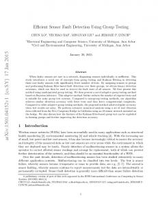
Fig. 1: The input of a GROTESQUE tests is a set of n items with unknown number of defectives. There are three possible outputs: there exists no defective item, or there exists exactly one defective item and the corresponding index number, or there exist at least two defective items (but GROTESQUE does not output the corresponding index numbers). There are two parts to GROTESQUE Encoding: the Multiplicity Encoder and the Localization Encoder. For the Multiplicity Encoder, we generate m1 tests. Each item is included in each test uniformly at random. In the Localization Encoder, whether or not a certain item is included in m2 tests is determined by the corresponding codeword of an expander code. The inputs to GROTESQUE Decoding are the results of outputs of GROTESQUE Encoding passing through BSC(q). Again, GROTESQUE Decoding is divided into two parts: the Multiplicity Decoder and the Localization Decoder. In the Decoder, we count the number of positive outputs of the Multiplicity Encoder, compare this number with the expected numbers for three cases, and decide on the multiplicity according to the rule given in Equation 1. We call the above process T HRES(.) (short for threshold detector). To implement the Localization Decoder, we use EXP DEC (short for expander code decoder) to do the decoding. If there exists exactly one defective item, the output should be one of the codewords of the expander code. This tells us which item is defective. The overall time complexity and error probability for the GROTESQUE tests are, respectively, O(log n) and O(1/poly(n)).

B. Localization If the multiplicity test estimates d to be 1, we then use the results of the m2 localization tests (which have been nonadaptively designed a priori) to localize the defective item. We represent the tests as a m2 × n matrix, A(L) . The difference between A(L) and A(M ) is that the columns of A(L) correspond to distinct codewords of an expander code, C (while the entries of A(M ) were chosen uniformly at random). Different columns correspond to different codewords. If there is exactly one defective item, then the output of the localization tests should be one of the codewords of C in the scenario with noiseless tests, or the result of one of the codewords of C XOR’d with a vector whose entries are i.i.d. Bernoulli(q) random variables in the scenario with noisy tests. By Theorem 1, the Localization step is correct with error probability ≤ 2−f m2 (where f is a constant for the code C) and decoding complexity O(m2 ). The following theorem about error-exponents of expander codes is useful in our construction. Theorem 1 ([31]): For a given rate R, any ε > 0, and α < 1 there exists a polynomial-time constructible code C of length m2 such that Pe (C, q) ≤ 2−αm2 f (R,

q)

, where

f (R, q) =

max

R≤R0 ≤1−H(q)

E(R0 , q)(R0 − R)/2 − ε

10

Here E(R0 , q) is the “random coding exponent” and H(·) is the binary entropy function. The decoding complexity of a sequential implementation of this decoding is O(m2 ) and f (R, q) is positive7 for all 0 < q < 1 − H(q).

C. Performance Analysis In this section, we analyze the error probability and time complexity of GROTESQUE tests in terms of m1 and m2 . The actual choices of these parameters are made in Sections IV, V and VI, corresponding respectively to our adaptive, non-adaptive, and two-stage algorithms. a) Error probability: We now bound from above the probability of error of the multiplicity and localization sub-routines of GROTESQUE testing. In Lemma 2 below, we explicitly derive the dependence of the probability of error of GROTESQUE tests on the value of q. This dependence can be directly translated into a dependence on the probability of error in each of our algorithms, but for ease of presentation we omit this dependence on q outside this lemma (and focus only on the dependence on D and N ).
2 Lemma 2: • The error probability of GROTESQUE multiplicity testing is at most exp −m1 (1 − 2q) /32 . •

Conditioned on d being correctly identified as 1, the error probability of GROTESQUE multiplicity testing is at most exp(−αm2 (1 − H(q))3 /128), for some universal α > 0.

Proof. Probability of error for multiplicity testing: The outputs of each individual test in the multiplicity testing are i.i.d. Bernoulli random variables, with mean depending on the value of d and q. There are three possible error events for multiplicity testing. 1) The true value of d equals 0, but GROTESQUE estimates it to be ≥ 1. In this scenario the expected number of positive outcomes is qm1 . To decide on the value of d (as either 0 or 1) the threshold that the multiplicity tester (given in Equation
1 is 21 q + 21 m1 . Hence the multiplicity tester makes an error if the true number of positive outcomes exceeds the

expected number by x1 = 12 q + 12 m1 − qm1 = m21 12 − q . 2) The true value of d equals 1, but GROTESQUE estimates it to be either 0 or at least 2. In this scenario the expected number of positive outcomes is m1 /2. To decide on the value of d (as either 1 or not) the closest threshold that the
multiplicity tester (given in (1) is 58 − 4q m1 . Hence the multiplicity tester may make an error if the true number of

positive outcomes differs from the expected number by x2 = 85 − 4q m1 − m21 = m41 12 − q . 3) The true value of d is greater than or equal to 2, but GROTESQUE estimates it to be either 0 or 1. In this scenario the
expected number of positive outcomes is at least 43 − 2q m1 . To decide on the value of d (as either ≥ 2 or not) the closest
threshold that the multiplicity tester (given in (1) is 85 − 4q m1 . Hence the multiplicity tester may make an error if the


true number of positive outcomes differs from the expected number by x3 = 43 − 2q m1 − 58 − 4q m1 = m41 21 − q . We now use the additive form of the Chernoff bound, which states that the probability of a m1 i.i.d. copies of a binary random variable differing its expected value by more than x is at most 2−2x analyzed, we have the desired bound on the probability of error. 7 In

[28], an improvement of this result is given without the constraints on q.

2

/m1

. Noting that x1 > x2 = x3 in the three cases

11

Probability of error for localization testing: This error event corresponds to the scenario when there is exactly one defective item and we claim that d = 1, but we locate the wrong defective item. Here we use the exponentially small outer bound on the probability of error of expander codes, as shown in Theorem 1, to bound our probability of error. The probability of error of the expander code is at most

Pe (C, q) ≤ 2−αm2 f (R,q) =

2−αm2 maxR≤R0 ≤1−H(q) E(R0 ,q)(R0 −R)/2− 2

≤ 2−αm2 (1−H(q)−R0 ) =

2−αm2 (1−H(q)−R)

≤ 2−αm2 (1−H(q))

3

3

(1−H(q)−R)/4

(2)

/16

/128

,

where for the middle inequality we choose R0 = (R + 1 − H(q)) /2, and the last inequality follows by choosing the rate R of our expander code to never be greater than (1 − H(q))/2. Based on the above analysis, setting m1 = O(log D) and m2 = O(log N ), we can guarantee that the error probability of GROTESQUE test is O(1/poly(N ) + 1/poly(D)). And in the setting D = Θ(N 1−δ ) which is of primary interest, the error probability scales O(1/poly(D)). b) Decoding complexity: Multiplicity testing only involves counting the total number of positives from m1 tests, and hence the complexity is O(m1 ). Localization testing involves decoding an expander code of block-length m2 , which is O(m2 ) by Theorem 1. IV. A DAPTIVE G ROUP T ESTING Adaptive Algorithm S Left subset, S ⊆ N degS (i) The number of neighbors in left subsets D-zero nodes {right nodes i: degD (i) = 0} D-leaf nodes {right nodes i: degD (i) = 1} D-non-leaf nodes {right nodes i: degD (i) ≥ 2} T The total number of stages (t) ∆ The set of unrecovered defectives before the t-th stage tests are performed, ∆(1) = D , t ∈ {1, . . . , T } (t) d The number of unrecovered defectives before the t-th stage tests are performed, d(t) = |∆(t) |, t ∈ {1, . . . , T } (t) G The bipartite graph for the t-th stage, t ∈ {1, . . . , T } r(t) The number of defectives recovered in t-th stage, r(t) = d(t) − d(t+1) , t ∈ {1, . . . , T − 1} TABLE IV: Table of notation used in our adaptive algorithm In this section, we consider the adaptive group testing problem. The objective here is to determine an unknown set D of D defective items from a collection N of size N . In this setting, we are allowed to perform tests sequentially in an adaptive manner, i.e., the subset tested in each test may depend on the outcome of previous tests. As stated earlier, we assume that each test outcome may be incorrect independently with probability q.

12

A. Overview

Fig. 2: In each t-th stage (t ≤ T − 1), we generate a bipartite graph with N nodes on the left representing N items and 2d(t) nodes on the right. The black circular nodes represent defective items and the white ones represent non-defective items. Each bipartite graph is left-regular with left-degree equal to 1. The left nodes of each such graph are partitioned randomly – different coloured collections show different “pools” within a partition. Nodes in the same pool connect to the same right node. Each right node passes the items connected to it to the GROTESQUE tests. If there exists only one defective in one pool, then GROTESQUE locates the defective item with high probability. For example, the second node in the red partition of first graph will be detected by the GROTESQUE tests at the first right node with high probability. In the next iteration, we exclude decoded defective items (colored blue) and use a similar decoding process. Finally, in the T -th stage, we generate a bipartite graph with c(log2 D)(log(log D)) right nodes. For each right node, we pick its c0 N log D neighbouring left nodes by choosing uniformly from all left nodes with replacement. By the coupon collection argument, with high probability, we can decode the remaining undecoded defective items.

Our algorithm has O (log(D)) adaptive stages. In all except the last stage, we design our tests so that with a high probability, in each stage, we recover a constant fraction of the remaining defectives. In each of these stages, the number of tests is roughly proportional to the number of remaining defectives. Thus, the total number of tests is O (D log N ). In each of these stages, the tests are designed by first removing the defectives recovered so far, partitioning the set of remaining items into twice as many sets as the number of remaining defectives, performing GROTESQUE tests on each set from the partition. In our analysis, to guarantee that in each stage we recover a constant fraction of the remaining defectives with a high enough probability, we apply concentration inequalities. This works only when the number of unrecovered defectives be at least Ω(log D). Thus, we move on to the last stage when all but log D defectives have been recovered. In the last stage, we use the coupon collection problem [30] as a primitive, to identify the remaining defectives. First we remove the set of defectives already recovered from the set of items being tested. Next, we design O (log D log log D) nonadaptive tests by picking random subsets of an appropriate size and performing GROTESQUE tests for that subset. We view the collection of outcomes from these sets of GROTESQUE tests as a random process that generates one independent “coupon” with constant probability each time. Thus, O (log D log log D) such tests suffice by standard coupon collector arguments. Overall, our algorithm requires O (D log N ) tests and runs in O (D log N ) steps.

13

B. Formal Description In this section, we describe an Adaptive Group Testing algorithm that achieves the following guarantees. Theorem 3: The Adaptive Group Testing algorithm described below has the following properties: 1) With probability 1−O(1/poly(D)) over the choice of the random bipartite graph, the algorithm produces a reconstruction ˆ of D such that D ˆ = D. of the collection D 2) The number of tests M equals O(D log N ) . 3) The number of stages is O (log(D)). 4) The decoding complexity is O(D(log(N )). Let ∆(t) , and d(t) , respectively be the set, and the number, of unrecovered defectives before the t-th stage tests are performed. Note that D = ∆(1) ⊇ ∆(2) . . . and D = d(1) ≥ d(2) ≥ . . . since we recover some defectives in each stage. Let T = 1 + inf{t : d(t) ≤ log D} denote the number of stages after which (with high probability) the number of unrecovered defectives is no larger than log D. For any right node i, and subset of left nodes S ⊆ N we define degS (i) as the number of left nodes that neighbor the right node i. There are three types of right nodes: D-leaf nodes, D-zero nodes and D-non-leaf nodes. A D-leaf node is a right node i with degD (i) = 1 (it is connected to a single defective item), a D-zero node is a right node i with degD (i) = 0 (it is connected to no defective items), and a D-non-leaf node is a right node i with degD (i) ≥ 2 (it is connected to multiple defective items). Specifically, D-leaf nodes are very helpful in our quick decoding process since our GROTESQUE black-box shall with high probability correctly output the location of a defective item if there exists exactly one defective item among its neighbours. Note: Even though in all our algorithms, both D-zero nodes and D-non-leaf nodes contain “potentially useful” information, we do not use them for decoding. This is because we require our algorithms to work with computational complexity that is comparable (up to constant factors for the adaptive algorithm, and at most a logarithmic factor in the other algorithms) to the size of the output of our algorithm (that is, O (D log(N ))). To run this “blindingly fast”, we need our algorithms to output “something interesting” in “very little” time. So, for instance, while the D-zero nodes tell us which inputs are non-defective, using this information takes “too long” (since it essentially tells us which items are not interesting rather than those which are interesting, but there are many more non-interesting items than interesting ones). a) Test design: Conceptually, we design the first T − 1 stages of our adaptive algorithm using the idea of “random binning”, and the T -th stage using that of “coupon collection”. •

Random binning: For each stage t = 1, . . . , T − 1, we consider a random left regular bipartite graph G (t) with 2d(t) right nodes and N − (D − d(t) ) left nodes corresponding to the set (N \ D) ∪ ∆(t) , i.e., all items except those already recovered in the previous t − 1 stages. We let each left node of G (t) be of degree one. We choose this graph uniformly at random from all possible bipartite graphs having mentioned properties above. Next, for each right node of G (t) , we use its set of left neighbours as the input for a GROTESQUE test. In each stage, for each right node of G (t) , if GROTESQUE detects it has multiplicity one, it decodes the corresponding defective item. Else if GROTESQUE identifies a right-node as having multiplicity greater than one or zero, it does not further use these test outcomes.

14

•

Coupon collection: In the final stage, we consider a left regular bipartite graph G (T ) with left node set (N \D)∪∆(T ) and c(log D)2 log log D right nodes. For each right node, we choose its c0 N/ log D neighbours independently and uniformly at random with replacement. Next, we design O (log N ) GROTESQUE tests at each right node to test for defectives among its O (N ) left neighbours.

b) Decoding algorithm: The decoding for each stage corresponds to detection of leaf nodes in that stage and corresponding localization via GROTESQUE tests. Specifically, in each of the t-th stages for t ≤ T , we sequentially pass the outputs of each of the right nodes of G (t) to GROTESQUE, which identifies leaf nodes and localized the corresponding defective items. Note that the structure of G (T ) at the T -stage differs from the structure of G (t) for t < T , since they are chosen according to different processes (coupon collection versus random binning). Nonetheless, the same decoding procedure (leaf detection and corresponding localization of defectives) is performed in both the first T − 1 stages, and th T th stage. The algorithm makes an error if not all defective items have been localized by the T -th stage (one can test for this by passing the set of remaining items to GROTESQUE’s multiplicity testing subroutine).

C. Performance Analysis To analyze the performance of the first part of the algorithm, we require the following lemma. Lemma 4: Let G be a random bipartite graph with n nodes on the left, and 2d nodes on the right side. Let ∆ be a subset of the left nodes of size d. Also, let each node on the left side of G have degree one. Then, for any  > 0, with probability at least 1 − exp(−2 d/2), at least (e−1/2 − )d nodes on the left are connected to ∆-leaf nodes. Proof. We first note that the probability that a node j ∈ ∆ on the left of the bipartite graph is connected to a ∆-leaf node is: Pr(j is connected to a ∆-leaf)



2d − 1 2d

d−1



1 1− 2d

(2d−1)/2

= >

where the last inequality comes from the well-known inequality: 1 −


1 x−1 x

> e−1/2 ,

> e−1 . Therefore the expected number of nodes

from ∆ that are connected to ∆-leaf nodes is e−1/2 d. Next, we show a concentration result for this number by applying McDiarmid’s inequality [29] the statement of which is reprised in Appendix A as follows. First, we label nodes on the right with numbers from 1 to 2d and for each i ∈ 1, 2, . . . , d, let Xi , label of the node on the right which is connected to the i-th node in ∆. Also, define f : X1 × X2 × · · · × Xd → Z as the number of left nodes connected to a ∆-leaf node i.e., f (x1 , x2 , · · · , xd ) , |{x1 , x2 , · · · , xd }|

(3)

15

It is observed that for any fixed x1 , · · · , xi−1 , xi+1 , · · · , xd and any xi , x0i ∈ Xi , |f (x1 , · · · , xi , · · · , xd ) − f (x1 , · · · , x0i , · · · , xd )| ≤ 2 For example, ∃i, j(6= i), xi = xj and x0i 6= xi . It’s possible that xj -th and x0i -th right nodes which initially are not ∆-leaf nodes become ∆-leaf nodes. Then, f (x1 , · · · , xi , · · · , xd ) − f (x1 , · · · , x0i , · · · , xd ) = −2. In fact, we can numerate all possible cases to conclude out result. It is clear that Xi ’s are independent. Therefore, by McDiarmid’s inequality we have:
Pr (f (X1 , X2 , · · · , Xd ) − Ef (X1 , X2 , · · · , Xd ) < −d) ≤ exp −2 d/2 . Hence,   ≤ Pr f (X1 , X2 , . . . , Xd ) − e−1/2 d < −d ≤

Pr (f (X1 , X2 , . . . , Xd ) − Ef (X1 , X2 , . . . , Xd ) < −d)
exp −2 d/2

Corollary 5: With probability 1 − O (exp (−D) + (log D)/N ), in each of the first T − 1 stages, our decoding algorithm recovers at least a e−1/2 /2 fraction of defectives that have not been decoded up to that stage. Proof. The event that we recover fewer than e−1/2 /2 fraction of defectives in t-th stage is a subset of the union of the following two events: (1) Less than a e−1/2 /2 fraction of defectives are connected to a ∆(t) -leaf node. (2) The outcome of the GROTESQUE tests is incorrect for any of the 2d(t) right nodes. By Lemma 4, with ∆ = ∆(t) , n = N − d(t) , and  = e−1/2 /2, the probability of event (1) is at most exp(−d(t) /4e). Further, by Lemma 2, with n = N − d(t) , the probability of event B is O (1/N ). For each t, let r(t) = d(t) − d(t+1) . Therefore, the probability that in one of the T − 1 stages, fewer than a e−1/2 /2 fraction of defectives are correctly decoded is bounded from above as 

−1 (t) Pr ∪Tt=1 {r

1 −1  TX e− 2 d(t) < e−1/2 d(t) /2} = Pr r(t) < 2 t=1

t−1 ( )! 1 \ e− 2 d(τ ) (τ ) r > . 2 τ =1

Under the conditioning event for the t-th term, we may bound d(t) from above by D(1−e−1/2 /2)t−1 . Further, by the definition of T , there are at most log D/ log (1 − e−1/2 /2) − 1 terms. The chain of inequalities is further simplified as   −1 (t) Pr ∪Tt=1 {r < e−1/2 d(t) /2}  1 −

log D/log (1− e

≤

 O 

X t=1

2

2



)−1

 exp (−D(1 − e−1/2 /2)t−1 ) + 1/N  

= O (exp (−D) + (log D)/N )

16

a) Number of tests: In the Random Binning part of the algorithm, there are 2d(t) right nodes in the t-th stage, each of which requires Cd(t) log N tests for some constant C = C(q) (as determined in Section III). Hence the total number of tests for the Random Binning PT −1 part of the algorithm is t=1 2Cd(t) log N . By Corollary 5, with high probability, in each stage the algorithms recovers a constant fraction of the undecoded defectives. Thus, d(t) = O (αt D) for some constant α ∈ (0, 1). Therefore, the total number of tests required in the first T − 1 stages is O (D log N ). For the Coupon Collection stage, the number of right nodes is O (log D log log D). Since we perform GROTESQUE tests for each right node, the total number of tests required is O (log D log log D log N ), which is less than the O (D log N ) tests required in the Random Binning part of the algorithm. Thus our proposed scheme requires O (D log N ) tests overall. b) Decoding complexity: Since in each stage our decoding algorithm has to step through all right nodes to decode the corresponding GROTESQUE PT −1 tests, the total number of right nodes the algorithm needs to consider is t=1 d(t) + O (log D log log D) = O (D). By the analysis from Section III-C, decoding each collection of GROTESQUE tests at a right node takes O (log N ) time. Therefore, our algorithm runs in O (D log N ) time. c) Error probability: We show that the above algorithm succeeds with high probability in decoding all the defectives in the claimed number of stages. By the analysis of error events (1) and (2) in Corollary 5, in the first part of the algorithm (random binning) we recover at least D − log D defectives with probability 1 − O (exp(−D) + (log D)/N ). To analyze the last (coupon collection) stage of tests, note that an error may occur only if one of the following events occur, (3) In the coupon collection process, fewer than log D distinct coupons are collected. (4) At least one of the collected coupons was incorrectly decoded. To bound the probability of event (3), we apply standard concentration bounds on the coupon collector’s problem [30]. Towards this end, we first note that the probability that our algorithm identifies a right node i as a leaf node may be written as Pr(i decoded as a ∆(T ) -leaf node) ≥ Pr(i decoded as a ∆(T ) -leaf node, i is a ∆(T ) -leaf node) =

Pr(i decoded as a ∆(T ) -leaf node | i is a ∆(T ) -leaf node) × Pr(i is a ∆(T ) -leaf node)

(1 − O (1/N )) × Pr(i is a ∆(T ) -leaf node) cN   log D cN log D log D = Θ(1) × 1− log D N − D + log D N − D + log D

=

=

Θ(1).

17

Since each decoded leaf node is independently chosen and the probability of picking a coupon is constant, by tail bounds on the coupon collection process [30], the probability that at least one coupon has not been collected in c0 (log D)2 log log D
steps is O (log D)− log D = O (poly(1/D)). Thus, the overall error probability decays as O (poly(1/D)). V. N ON - ADAPTIVE A LGORITHMS Non-adaptive Algorithm Gg g-th sub bipartite graph, g ∈ {1, . . . , c1 log D} ˆi y The length-O(log N ) binary vector denoting the actually observed noisy outcomes of the i-th GROTESQUE Encoding c1 A constant related to the number of sub bipartite graph c2 A constant related to the number of right nodes for each bipartite graph c3 A constant related to the number of multiplicity tests for each right node c4 A constant related to the number of localization tests for each right node c5 c5 = c1 c2 P0 The probability that the neighbor of a defective item is a D-leaf node L(D) Leaf node list which contains all the D-leaf nodes L(t) Leaf node list for the t-th iteration. Mi,1 The number of Multiplicity tests for right node i Mi,2 The number of Localization tests for right node i TABLE V: Table of notation used in our Non-adaptive algorithm

We consider non-adaptive group testing in this section. In non-adaptive group testing, the set of items being tested in each test is required to be independent of the outcome of every other test [11]. The objective here is to determine an unknown set D of D defective items from a collection N of size N . We assume that each test outcome may be incorrect independently with probability q.

A. Overview The structure of group-testing tests is based on left-regular bipartite graphs {Gg }. We put N items on the left-hand side and c5 D log D nodes on the right-hand side of a bipartite graph. Each node on the right-hand side of a bipartite graph is called a group-testing node. Group tests corresponding to the multiplicity and localization tests of GROTESQUE are performed as part of the encoding process, but the results are not necessarily used to decode. This is because our decoding algorithm can cherry-pick the group-testing nodes to decode only the “useful” ones. The set of D-leaf nodes (see the definition in Section IV-B) are helpful for our decoding process since GROTESQUE tests performed on a right node output the location of a defective item only if there exists exactly one defective item among its neighbours. In our iterative algorithm, we claim that there exists at least one D-leaf node in each iteration, so that we can decode one defective item.

B. Formal Description In this section, we describe a probabilistic construction of the tests and an iterative Non-Adaptive Group Testing algorithm that achieves the following guarantees.

18

Fig. 3: We generate c1 log D bipartite graphs with N nodes on the left (representing N items) and c2 D nodes on the right. Take G1 as an example. For each right node i, we generate O(log N ) tests, yˆi , by GROTESQUE tests. The input of the i-th GROTESQUE TESTS are the items connected to the right node i. The size of outputs is O(log N ). Based on the properties of GROTESQUE TESTS, we can estimate whether there exists exactly one defective item and if so, we can estimate its location with high probability.

Theorem 6: The Non-Adaptive Group Testing algorithm described below has the following properties: 1) With probability 1−O(1/poly(D)) over the choice of the random bipartite graphs, the algorithm produces a reconstruction ˆ of D such that D ˆ = D. of the collection D 2) The number of tests M equals O(D log D log N ). 3) The decoding complexity is O(D(log(N ) + log2 D)). a) Description of graph properties: We first construct a bipartite graph G (Figure 4) with some desirable properties outlined below. We then show that such the random graphs we choose satisfy such properties with high probability. In Section V-Bb), we then use these graph properties in the Non-adaptive Group Testing algorithm. Properties of G : 1) Construction of a left-regular bipartite graph: As in Figure 4, we generate G by combining c1 log D left-regular graphs Gg , for g = 1, . . . , c1 log D. For each Gg , there are N items on the left and c2 D group-testing nodes on the right. The graph Gg has left-regularity equal to 1 and each edge connects to a right node uniformly at random. After constructing all the c1 log D graphs Gg , we combine them to form G in the following way. Keep N items on the left, and collect the right nodes. Therefore, G has the properties that it has N nodes on the left with left-regularity equal to c2 log D, and c5 D log D = c1 c2 D log D nodes on the right.

19

Fig. 4: After generating c1 log D bipartite graphs as in Figure 3, we combine them to obtain the overall graph G for our non-adaptive group testing algorithm. There are N nodes on the left representing N items. Collect the right nodes of all the c1 log D bipartite graphs on the right side of G and maintain the connectivity between two sides. Different colors show the connectivity between N items and different right node sets of equal size c2 D. Finally, we get a bipartite graph G with left regularity equal to c1 log D. We can guarantee that, with high probability, each defective item connects to a D-leaf node.

2) “Many” D-leaf nodes: For any set D of size D on the left of G, none of the nodes in D has fewer than a constant fraction of D-leaf nodes. The proof of this statement is the subject of Lemma 7. Lemma 7: With probability 1 − O(D−1 ), the fraction of c1 log D neighbors of each defective item that are D-leaf nodes is Ω( exp(−1/c2 )) .

20

Proof. Define Wi,j as the random variable representing whether the neighbor of a defective item xj is a D-leaf node for the i-th graph Gi . Wi,j =

   1, if the neighbor left node j is a D-leaf node   0,

otherwise

Then, the total number of D-leaf nodes of xj is

P0

Plog D

,

= ≈

i=1

Wi,j .

Pr(the neighbor of a defective item xj is a D-leaf node) D−1  1 1− c D  2  1 exp − , c2

and W1,j , . . . , Wc1 log D,j are i.i.d. Bernoulli random variables with parameter P0 . Therefore, by the Chernoff bound, we have Pr

c1X log D

! Wi,j − P0 c1 log D ≤ −P0 c1 log D

i=1 2

≤

   exp − P0 c1 log D 2

Hence, the probability for each defective item that it has at least a constant fraction of D-leaf nodes is 1 − O(1/D) (by choosing the c1 and c2 appropriately). Then, by the union bound, all defective items have at least constant fraction of D-leaf nodes. In the following two sections, we describe how to use the properties of G to perform the encoding and decoding. b) Test design: For each node i on the right of G, we design GROTESQUE tests with degN (i) inputs which are the items connected to right node i. We choose the number of multiplicity tests, Mi,1 , equal to c3 log(c5 D log D) and the number of localization tests, Mi,2 , equal to c4 log(degN (i)) for some positive constant c3 and c4 . We already know that c3 log(c5 D log D) = O(log D). Since the right degree of any node is at most N , the total number of GROTESQUE-tests required for the right node i equal to Mi,1 + Mi,2 = O(log N ). Therefore, the overall number of tests M equals O(D log D log N ). c) Decoding algorithm: Before the iterative decoding process, we make a leaf node list, L(D), which contains all the D-leaf nodes based on the multiplicity testing part of GROTESQUE tests. Based on the properties of graph G, we know that each defective item has at least a constant fraction of D-leaf nodes. Denote L(t) as the leaf node list in t-th iteration, t = 1, 2, . . . , D, D +1. L(1) = L(D), L(D+1) = ∅ and L(t) 6= ∅, for t = 1, 2, . . . , D. In the t-th iteration, we pick a right node i ∈ L(t) and decode a defective item using the localization part of GROTESQUE tests of i to locate the corresponding defective item. After that, we cancel the defective item, its corresponding edges and its neighbors. We update the L(t) to L(t+1) . In the (t + 1)-th iteration, we pick

21

another D-leaf node in L(t+1) . The formal description of the non-adaptive group testing algorithm is as follows: 1) Initialization : Go through all the right nodes and use only the multiplicity testing part of GROTESQUE-test to initialize L(1) = L(D). 2) Operations in t-th iteration : i) Pick any right node j in L(t) ; ii) Use localization part of GROTESQUE-test to decode the corresponding defective; iii) Remove the decoded defective item, all the edges connected to it, and all its neighbours; iv) Update L(t) to L(t+1) by removing the leaf nodes removed in step iii) and return to step i). ˆ 3) T ermination : The algorithm stops when the leaf node list becomes empty, and outputs the defective set D.

C. Performance Analysis a) Number of iterations: Since we guarantee that in each iteration we can decode one defective item, the number of iterations is D. b) Decoding complexity: For each right node, checking the multiplicity testing part of GROTESQUE-test costs c3 log(c5 D log D) steps. Therefore, the total computational cost is [c3 log(c5 D log D)](c5 D log D) = O(D log2 D) in the initialization step. In each iteration, the cost of localization is O(log N ) steps. Removing the decoded defective item takes 1 step. Removing all the edges connected to it and its neighbours takes time log(c5 D log D)](c1 log D) = O(log2 D), where log(c5 D log D) is the cost of addressing one neighbour of the decoded defective item. Therefore, the time complexity for the iterative decoding process is O(D(log N + log2 D)). Hence, we can conclude that the overall time complexity is O(D(log N + log2 D)) based on the analysis above. c) Error probability: ˆ = D with a high probability by choosing the parameters c3 and c4 carefully. Finally, we show that D We set Mi,1 = c3 log(c5 D log D) to make sure that the probability of incorrect multiplicity decoding for each node is O(1/c5 D log D) by choosing c3 > 1. Then by the union bound, the probability of incorrect multiplicity decoding is O (1/poly(D)). We set Mi,2 = c4 log(degN (i)) = O(log N ) to make sure that each neighbour of i has distinct codewords by choosing c4 > 1. The probability of incorrect localization in each iteration is O(exp(−Mi,2 )) which is upper bounded by O(1/N ). Finally, by applying the union bound over D iteration, the probability of incorrect decoding is bounded from above by O (1/poly(D)). VI. T WO - STAGE GROUP TESTING In this section, we present a 2-stage adaptive group testing problem with both decoding complexity and number of tests that is nearly order-optimal (up to a multiplicative factor that is at most O (log N )). Again, the objective is to determine an unknown set D of D defective items from a collection N of size N . In both stages, we perform tests in a non-adaptive manner,

22

though the tests of the second stage depend on the outcomes of tests in the first stage. As earlier, we assume that each test outcome may be incorrect independently with probability q.

A. Overview

Fig. 5: In the first stage, we generate a bipartite graph with N nodes on the left representing N items and S nodes on the right. The black circular nodes represent defective items and the white ones represent non-defective items. Each bipartite graph is left-regular with left-degree equal to 1. The left nodes of such graph are partitioned randomly – different coloured collections have different “birthdays”. Nodes in the same partition have the same “birthday”. With high probability, each right node is either D-leaf node (black right node) or D-zero node (white right node) according to our choice of S. Applying our non-adaptive algorithm, we identify D leaf nodes. In the second stage, applying localization testing on each D-leaf node, we identify the corresponding defective items.

Two-Stage Adaptive Algorithm G A bipartite graph used in the first stage S The number of nodes on the right of G TABLE VI: Table of notation used in our 2-stage adaptive algorithm

Our algorithm has 2 adaptive stages. In the first stage, we use the birthday paradox problem as a primitive to construct a bipartite graph G. G has the following properties - the graph is bipartite, has N nodes on the left representing N items (N “people”), is left-regular with regularity equals 1, and S (= poly(D) with degree larger than 3) nodes on the right (S choices of “birthdays”). We show that with high probability (1 − O (1/poly(D))), each right node is either a D-leaf node or a D-zero node (i.e., no pair of them have the same birthday). We use the non-adaptive algorithm discussed in Section V on the S right nodes to identify the D Dleaf nodes. In the first stage the total number of tests is O(D log D log S) = O(D log2 D) and the decoding complexity is O(D(log S + log2 D)) = O(D log2 D).

23

In the second stage, we use the localization procedure of GROTESQUE with n = O ((N/poly(D))), on all D-leaf nodes identified in the first stage. Note that with high probability there are exactly D right nodes that are D-leaf nodes, out of poly(D) right nodes in total – the fact that we test only D of them is what gives us potentially significant savings in the number of tests and decoding complexity. In the second stage the total number of tests is O(D log N ) and the decoding complexity is O(D log N ). Over both stages, our 2-stage adaptive algorithm hence requires O(D(log N + log2 D)) tests and runs in O(D(log N + log2 D)) steps.

B. Formal Description In this section, we describe a 2-stage adaptive group testing algorithm that achieves the following guarantees. Theorem 8: The Two-stage Adaptive Group Testing algorithm described below has the following properties: 1) With probability 1−O(1/poly(D)) over the choice of the random bipartite graph, the algorithm produces a reconstruction ˆ of D such that D ˆ = D. of the collection D 2) The number of tests M equals O(D(log N + log2 D)). 3) The number of stages is 2. 4) The decoding complexity is O(D(log N + log2 D)). a) Test design and decoding algorithm: •

Birthday paradox hashing: In the first stage, we consider a random left regular bipartite graph G with S right nodes and N left nodes. We set each left node of G to be of degree one. We choose this graph uniformly at random. The property we required is that, with high probability, each right node is either a D-leaf node or a D-zero node (see the definitions in Section IV-B). By the “standard birthday paradox argument” [32], the failure probability scales as O(1/poly(D)) if we choose S = O(poly(D)) with degree larger than 3 (see Lemma 9 below). To identify all the D-leaf nodes is equivalent to the group testing problem of finding D defectives from S items. We apply our non-adaptive algorithm to all right nodes. Here if a right node i is (respectively is not) included in a test, then all the neighbors of i are (respectively are not) included in that test. The outcomes of the first stage are all D-leaf nodes.

•

Localization: In the second stage, we use the GROTESQUE localization procedure (with n = O (N/poly(D))) on each D-leaf node identified in the first stage, to decode the corresponding defective item.

C. Performance Analysis The analyze the performance of the first part of the algorithm, we require the following lemma. Lemma 9: The probability that no defective items have the same neighbor (right node) scales as 1 − O(1/poly(D)), if we choose S = O(poly(D)) with degree larger than 3. Proof. There are at least two ways to prove the correctness of this lemma.

24

First, using an argument similar to that in the birthday paradox problem, Pr(No defective items have the same neighbor)
S D D! = D S     1 2 D−1 = 1− 1− ... 1 − S S S   D−1 Y i = 1− S i=1 Using 1 −

i S

≈ e−i/S when i  S,

D−1 Y i=1

i 1− S

 ≈

D−1 Y

e−i/S

i=1 P − D−1 i=1 i/S

=

e

=

e−D(D−1)/2S

≈

e−D

≈

1−

2

/2S

D2 2S

Therefore, if we choose S = O(poly(D)) with degree larger than 3, the probability that each right node has no more than two defective items is 1 − O(1/poly(D)). For an alternative proof, we consider the probability that the event considered in the statement of this lemma does not happen. The probability Pr(Any two defective items have the same neighbor) equals S1 . Then, by the union bound, the probability 2 (D) that there exist two defective items that have the same neighbor is at most S2 < DS . Again, we choose S = O(poly(D)) with degree larger than 3 to complete the proof. a) Number of tests: The number of tests in the first stage is O(D log D log S) = O(D log2 D) and the number of tests in the second stage is O(D log N ). Overall, the number of tests required is O(D(log N + log2 D)). b) Decoding complexity: The decoding complexity in the first stage is O(D log S + D log2 D) = O(D log2 D) and the decoding complexity in the second stage is O(D log N ). Overall, the decoding complexity is O(D(log N + log2 D)). c) Error probability: There are three events we need to consider. First, the error probability of constructing bipartite graph G with the properties we need is O(1/poly(D)). Second, the error probability of non-adaptive group testing algorithm is O(1/poly(D)). Third, the error probability of any localization testing is O(1/N ). By applying union bound over D D-leaf nodes, the probability of incorrect decoding is O(1/poly(D)).

25

Therefore, the overall error probability of incorrect decoding scales as O(1/poly(D)). VII. C ONCLUSION In this work we consider three group testing algorithms, specifically for adaptive, nonadaptive, and two-stage adaptive scenarios. In each of these scenarios, we present the first algorithms whose computational complexity is nearly informationtheoretically order-optimal. The number of tests required in our algorithms is also nearly information-theoretically order-optimal (by the same factor). VIII. A PPENDIX A. Mcdiarmid’s Inequality Let X1 , . . . , Xm be independent random variables all taking values in the set X . Further, let f : X m 7→ R be a function of X1 , . . . , Xm that satisfies ∀i, ∀x1 , . . . , xm , x0i ∈ X ,

|f (x1 , . . . , xi , . . . , xm ) − f (x1 , . . . , x0i , . . . , xm )|

≤ ci

Then for all  > 0,

 Pr (f − E [f ] ≥ ) ≤ exp

−22 2 Σm i=1 ci



and  Pr (f − E [f ] ≤ −) ≤ exp

−22 2 Σm i=1 ci



R EFERENCES [1] V. Guruswami and P. Indyk, “Linear-time list decoding in error-free settings: (extended abstract),” in ICALP, 2004, pp. 695–707. [2] P. Indyk, H. Ngo, and A. Rudra, “Efficiently decodable non-adaptive group testing,” Proceedings of the Twenty-First Annual ACM-SIAM Symposium on Discrete Algorithms, pp. 1126–1142, 2010. [3] H. Ngo, E. Porat, and A. Rudra, “Efficiently decodable error-correcting list disjunct matrices and applications,” in Automata, Languages and Programming, ser. Lecture Notes in Computer Science, 2011, vol. 6755, pp. 557–568. [4] M. Sobel and R. M. Elashoff, “Group testing with a new goal, estimation,” Biometrika, vol. 62, no. 1, pp. 181–193, 1975. [5] R. Dorfman, “The detection of defective members of large populations,” Annals of Mathematical Statistics, vol. 14, pp. 436–411, 1943. [6] M. T. Goodrich and D. S. Hirschberg, “Improved adaptive group testing algorithms with applications to multiple access channels and dead sensor diagnosis,” Journal of Combinatorial Optimization, vol. 15, pp. 95 – 121, Jan 2008. [7] J. Wolf, “Born again group testing: Multiaccess communications,” Information Theory, IEEE Transactions on, vol. 31, no. 2, pp. 185 – 191, mar 1985. [8] H. Q. Ngo and D.-Z. Du, “A Survey on Combinatorial Group Testing Algorithms with Applications to DNA Library Screening,” in DIMACS Series in Discrete Mathematics and Theoretical Computer Science, vol. 55, 2000, pp. 171 – 182. [9] A. Schliep, D. Torney, and S. Rahmann, “Group testing with dna chips: generating designs and decoding experiments,” in Bioinformatics Conference, 2003. CSB 2003. Proceedings of the 2003 IEEE, aug. 2003, pp. 84 – 91. [10] Y. Cheng and D. Du, “New constructions of one- and two-stage pooling designs,” Journal of Computational Biology, vol. 15, no. 2, pp. 195–205, 2008.

26

[11] D. Du and F. K. Hwang, Combinatorial Group Testing and Its Applications, 2nd ed.

World Scientific Publishing Company, 2000.

[12] D. Z. Du and F. K. Hwang, “Combinatorial group testing and its applications,” World Scientific Series on Appl. Math, 1999. [13] M. B. Malyutov, “Separating property of random matrices,” Mat. Zametki, vol. 23, pp. 155–167, 1978. [14] C. L. Chan, P. H. Che, S. Jaggi, and V. Saligrama, “Non-adaptive probabilistic group testing with noisy measurements: Near-optimal bounds with efficient algorithms,” in 49th Annual Allerton Conference on Communication, Control, and Computing (Allerton), 2011. [15] E. Porat and A. Rothschild, “Explicit non-adaptive combinatorial group testing schemes,” in Automata, Languages and Programming, ser. Lecture Notes in Computer Science, 2008, vol. 5125, pp. 748–759. [16] A. Mazumdar, “Construction of almost disjunct matrices for group testing,” Apr 2012. [17] M. B. Malyutov and H. Sadaka, “Jaynes principle in testing active variables of linear model,” Random Operators and Stochastic Equations, vol. 6, pp. 311–330, 1998. [18] G. Atia and V. Saligrama, “Boolean compressed sensing and noisy group testing,” IEEE Transactions on Information Theory, vol. 58, pp. 1880 – 1901, March 2012. [19] F. K. Hwang, “Group testing with a dilution effect,” Biometrika, vol. 63, no. 3, pp. pp. 671–673, 1976. [20] A. De Bonis, L. Gasieniec, and U. Vaccaro, “Optimal two-stage algorithms for group testing problems,” SIAM Journal on Computing, vol. 34, no. 5, pp. 1253–1270, 2005. [21] M. M`edzard and C. Toninelli, “Group testing with random pools: Optimal two-stage algorithms,” Information Theory, IEEE Transactions on, vol. 57, no. 3, pp. 1736 –1745, march 2011. [22] P. Damaschke and A. S. Muhammad, “Randomized group testing both query-optimal and minimal adaptive,” in Proceedings of the 38th international conference on Current Trends in Theory and Practice of Computer Science, ser. SOFSEM’12, 2012, pp. 214–225. [23] A. G. Dyachkov and V. V. Rykov, “Bounds on the length of disjunctive codes,” Probl. Peredachi Inf., vol. 18, pp. 7–13, 1982. [24] A. G. Dyachkov, V. V. Rykov, and A. M. Rashad, “Superimposed distance codes,” Problems Control Inform. Theory, vol. 18, pp. 237 – 250, 1989. [25] G. Cormode and S. Muthukrishnan, “What’s hot and what’s not: tracking most frequent items dynamically,” ACM Trans. Database Syst., pp. 249–278, 2005. [26] M. T. Goodrich, M. J. Atallah, and R. Tamassia, “Indexing information for data forensics,” in ACNS’05, 2005, pp. 206–221. [27] D. A. Spielman, “Linear-time encodable and decodable error-correcting codes,,” in STOC, 1995, pp. 388–397. [28] A. Barg and G. Z´emor, “Error exponents of expander codes under linear-complexity decoding,” SIAM Journal on Discrete Mathematics, vol. 17, no. 3, pp. 426–445, 2004. [29] C. McDiarmid, “On the method of bounded differences,” Surveys in combinatorics, vol. 141, no. 1, pp. 148–188, 1989. [30] R. Motwani and P. Raghavan, Randomized Algorithms.

Cambridge University Press, 1995. [Online]. Available: http://books.google.com/books?id=

QKVY4mDivBEC [31] A. Barg and G. Zemor, “Error exponents of expander codes,” Information Theory, IEEE Transactions on, vol. 48, no. 6, pp. 1725 –1729, jun 2002. [32] W. Feller, An Introduction to Probability Theory and Its Applications. Vol. I, 2nd ed. Wiley, New York, 1958.