GROUNDWATER FLOW MODELING WITH UNCERTAIN DATA

GROUNDWATER FLOW MODELING WITH UNCERTAIN DATA M. Maradjieva The University of Architecture, Civil Engineering and Geodesy, Sofia, Bulgaria

O. Georgieva Institute of Control and System Research- BAS, Sofia, Bulgaria

ABSTRACT: The joint model for surface and subsurface water interaction has been applied for the case of pumping well near small river. The variability of transmissivity has been assessed using fuzzy technics. The model has been applied for the case of 2-D hydrogeological river-aquifer interaction. The results show the importance of two fuzzy models for construction of the field of transmissivity in the examinated area. On the base of expert knowledge and a set of fuzzy rules, this field would be constructed and used in numerical modeling.

1 INTRODUCTION The most complex problems concerning water supply require taking into account the integrity of surface and subsurface water. The river flow is influenced from natural and artificial factors acting on the catchment area. The groundwater extraction causes the reduction in water discharge downstream and temporary distribution of the river flow as well. This effect could be significant for small rivers during the low flow periods. The modern approach requires to assess the influence of engineering structure on the environment. This is often the case of downstream hydropower dam station with hydropeaking unstable flow regime or extended water consumption for agriculture, farming or water supply. This unfavorable seasonal distribution is also related to the ecological integrity, physical aquatic habitat and the aquatic ecosystem dynamics. For ecological purposes the threshold discharge must be ensured to protect the aquatic ecosystem of the river. It is obvious that rational use of water resources requires application of joint model for surface and

subsurface water. It is necessary especially for the case of pumping well near a small river, where the impact between river and groundwater is significant. The uncertainty of some hydrogeological parameters reflects directly on the model results, so sensitivity analysis has to be implemented in the model. 2 DESCRIPTION OF THE JOINT MODEL Two models are presented herein: unsteady model for simulation of hydrological process in the river and 2-D joint model for surface and subsurface dynamics. An unsteady wave movement can be described by the equations for 1-D open channel flow known as St. Venant equation ( Piren-Seine, Rapport de synthese, 1989-92, vol. II ). ∂A ∂Q + =0 (1) ∂t ∂x ∂Q ∂ ⎛ Q2 ⎞ ∂h ⎟ + gA + gA (S f − S ) = 0 + ⎜β (2) ∂t ∂x ⎜⎝ A ⎟⎠ ∂x

where x is the distance in downstream direction, t is time, A is wetted cross-sectional area, h is the depth of the flow, S is bed slope of the β is momentum correction channel, coefficient(≈1), Sf is friction slope, Q is the discharge. Because of their complexity the equations (1) and (2) are more rarely used in the joint models. Moreover in most natural rivers, there are some simple assumptions. If the inertial terms in the momentum equation are so small to be negligible in comparison with the bed slope term, the above two equations can be reduced to a convective-diffusion equation (Cunge, J.A. et al. 1985). ∂Q ∂Q ∂ 2Q +c = D 2 + cq (3) ∂t ∂x ∂x where c(x,t) is the velocity describing the translation characteristics of the wave, D is the diffusion coefficient, q is the lateral increment of discharge per unit length of x (q>0 in direction towards the river, otherwise- towards the riverbanks). If both inertial and pressure forces are neglected, the St. Venant equations give the kinematic wave equation (Cunge, J.A. et al. 1985). ∂Q ∂Q +c =0 (4) ∂t ∂x Due to the physical nature of the hydrological process in the river convectivediffusion equation (3) was chosen for the description of the joint model. For assessment of the parameters D and c in (3) the following simplification are used: 1 ∂Q c= (5) b ∂h Q D= (6) 2bS f where b is the with of the river, D is the diffusion coefficient, Sf is the friction slope. If the explicit scheme is applied, the stability condition must be satisfied: Δt C0 = c ≤1 (7) Δx where C0 is the Courant number. The implicit schemes are effective in overcoming the stability criterion or equivalent

ones. The following initial and boundary condition were used: Q (x,0) =Q0 (8) t =0 The upper and the lower boundary conditions are as follows: Q (0,t)=Q(t) (9) x =0 ∂Q =0 (10) ∂x As a rule the rating curve can be used for determination of the head in the river flow: (11) Q =α (h+h*)β

x=L

where h is the piezometric head in the river,

α and β are the coefficient of the curve.

Considering the mass balance of water in a volume of soil height b and two directions dx and dy, one obtains the continuity equation: ∂H ∂ ⎛ ∂H ⎞ ∂ ⎛ ∂H ⎞ ⎟=S ⎜T ⎟ + ⎜T (12) ∂t ∂x ⎝ ∂x ⎠ ∂y ⎜⎝ ∂y ⎟⎠ where S and T are the storage coefficient and the transmissivity of the aquifer, His the piezometric head. For homogeneous isotropic soil, S and T are constant in a confined saturated aquifer. The joint model presents a set of 2-D hydrogeological part with equation (12) attached to the river with hydrodynamic partsee equations(3),(11). The use of the transmissivities between nodes allows the anisotropy to be included (Kinzelbach, W. 1986). To solve the nodal equations iteratively the IADI method ( Iterative Alternating Direction Implicite procedure ) was used with two tridiagonal systems: A′j Hij-1(t+Δt)+B′j Hij(t+Δt)+ (13) +C′j Hij+1(t+Δt)=D′j where j=1,NY and i=1,NX AiHi-1j(t+Δt)+BiHij(t+Δt)+ (14) +CiHi+1j(t+Δt)=Di After simplification the row-equations have the form: (15) Hij + Fi Hi+1j=Gi where Fi and Gi are recursively defined arrays as follows: Ci D − Ai Gi −1 , Gi = i Fi = (16) Bi − Ai Fi −1 Bi − Ai Fi −1

and , i=2,NX-1 The solution of the system has the following form: (17) H NXj (t + Δt ) = G NX H ij (t + Δt ) = Gi − Fi H i +1 j (t + Δt )

(18)

for i=NX-1,2 The similar form has the system of column equations. 3 SENSITIVITY ANALYSIS FOR SEMICONFINED AQUIFER The method for sensitivity assessment proposed by Guinot (1998) for the case of unconfined aquifer, is modified below for the case of confined or semi-confined aquifer. The differential equation for twodimensional modeling ( x1 and x 2 are coordinates of the field) of water movement in confined or semi-confined aquifer is: ∂H ∂2H =T μ (19) ∂t ∂xi2 where H is the piezometric head, T is the transmissivity and μ is the storage coefficient of the aquifer. Any perturbation in transmissivity τ will generate a perturbation in the solution η: (20) T ′ = T +τ H ′ = H +η

The perturbated solution Equation(19). ∂H ′ ∂2H ′ =T′ μ ∂t ∂x i2

(21) still

obeys

(22)

Subtracting Equation (19) from Equation (22) yields: ∂η ∂ 2η ∂2H = (T + τ ) 2 + τ μ (23) ∂t ∂xi ∂xi2 The result equation is not a transport equation as it is for the case of unconfined aquifer. For prescribed head-type boundary conditions, since the hydraulic head is assumed known exactly, η=0 at the boundary. For the

boundary of prescribed flux the followings relations are valid: (T + τ )ni ∂η = τ q (24) ∂xi T where n1 and n2 are the components of the vector normal to the boundary, q is prescribed flux. The sensitivity of the result piezometric head H at point M to the value of the input parameter T at point N is defined as: 1 η (M , t ) S HT = (25) A τ (N ) where A is the area of the perturbated region. 1 ∂S HT ∂ 2 S HT ∂2H = (T + τ ) +τ 2 (26) ∂t ∂xi ∂xi2 Aτ (N ) This equation allows making sensitivity analysis of transmissivity on computed heads. The value of sensitivity for the flux boundary conditions is derived as T (T + τ )n ∂S H = 1 q (27) ∂xi AT

μ

4 FUZZY MODELING OF THE FIELD OF TRANSMISSIVITY In order to model water transport a proper knowledge of the soil hydraulic properties, namely the transmissivity function T(.) is required. The task is to assess the field transmissivity in a certain area under given boundary conditions and imprecise knowledge of soil properties (e.g. porosity, grain distributions, etc.). Usually the distances between the point and the river are known exactly. In this case the transmissivity of the x coordinate is denoted by Tx , of the y coordinate - by Ty and by Txy when the transmissivity is equal in both directions. These relations could be defined deterministically using the following equations: n

Tx =

∑ kibi fix i =1

n

∑ fix i =1

n

, Ty =

∑ kibi fiy i =1

n

∑ fiy i =1

(28) (29)

n

Txy =

∑ kibi fixy i =1

n

∑ fixy

(30)

i =1

where ki is the hydraulic conductivity in the ith layer; bi is the thickness of the ith layer; fix, fiy, fixy, are weight coefficients and i=1,n is the number of ground layers. The expert information for the number, thickness and soil properties of the ground layers is quite vague. Therefore the resulting mean field transmissivity assessment by equations (28)-(30) is imprecise. Hence the transmissivity could be defined in the terms of fuzzy linguistic model (FLM) consisting a set of Ri, i=1,n “If-Then” linguistic rules: Ri: If the current point is on a distance bi* from the groundwater table, then the corresponding transmissivities are Tix , Tiy , Tixy where the distance bi* and field transmissivities Tix , Tiy , Tixy, for i=1,n are fuzzy sets. With expert knowledge for the soil and the thickness of the layers suitable fuzzy sets could be defined. They are implemented in the premise part of the rules Ri of the fuzzy model. The generalized bell membership function is preferred to define the premise fuzzy values of the following two case studies, which correspond to the realistic smooth changes of the ground layers. The field of transmissivity of every layer is estimated by corresponding equation (28),(29) or (30). Triangle symmetrical fuzzy sets are proposed on the base of obtained values. Every rule defines the real situation that the layer thickness is not exactly known. Its size and soil property varies by uncertain way, which defines different values of the transmissivity of the considered point. The centroid defuzzification method is applied. In case that the conductivity values of all layers are known sufficient precisely the Takagi-Sugeno (TS) fuzzy model could be applied. It consists of a set of n rules with consequent parts defined by single tones (constant values) equal to the corresponding transmissivities.

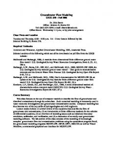
Example 1: Using the procedure given above a four rule fuzzy linguistic model were defined for the case study of symmetrical position (Figure 1). The fuzzy value of the field of transmissivity is obtained for every given depth by max-min composition rule of inference. The same experimental data are used to define the TS fuzzy model (Figure 2). The obtained numerical results of distance point 0.1 [m] from groundwater table are presented on Table 1. Table 1. Model

Tx [m2/d] 1.93 1.9

Ty [m2/d] 2.23 2.21

Txy [m2/d] 1.64 1.6

FLM TS model *Deter. model 1.846 2.143 1.5575 * Deterministic model by eqs. (28), (29), (30) Example 2: Using the procedure given above a three rule fuzzy linguistic model and TS fuzzy model were defined for the case study of nonsymmetrical position. The numerical results of point on distance 0.1 [m] from groundwater table are shown on Table 2. Table 2. Model

Tx [m2/d] 4.95 4.8

Ty [m2/d] 5.45 5.35

Txy [m2/d] 4.15 3.83

FLM TS model *Deter. model 4.55 5.14 3.531 * Deterministic model by eqs. (28), (29), (30)

The main advantage of the fuzzy models approach consists in overcoming of the need of large amount of field experiments. On the base of expert knowledge and a set of fuzzy rules two type fuzzy models of the transmissivity field could be constructed.

Figure 1: View rules of fuzzy linguistic model applied on point depth 1.5 [m] from groundwater table.

Figure 2: View rules of TS fuzzy model applied on point depth 1.5[m] from groundwater table.

x,y

5 RESULTS

sand clay loam1 loam2

2 x

well2

groundwater table Figure 4: Soil structure near the river.

well1

Table 3. Soil

4

q=const

2m

river

1

soil surface z 2m 1m 2m

The model was applied for the layered soil profile near the river. The initial conditions are given by: t=0, H(x,y,0)=H0(x,y) for all indices i=1,…,NX and j=1,…,NY Boundary conditions for unconfined aquifer are shown in figure 3.

Conduc Height tivity cm cmd-1

weight

fix

fiy

fixy

Sand

200

150

0.4

0.5 0.25

Clay

100

3

0.2

0.1 0.25

Loam1

200

90

0.2

0.2 0.25

Loam2

200

70

0.2

0.2 0.25

3

y Figure 3: Boundary conditions for joint model: 1-2 First kind boundaries with prescribed head: H0(x,y)=f(t) , for every t 1-4 Second kind with zero flux 2-3 Second kind with zero flux 4-3 Third kind with leakage boundary (semi-impervious ) Using the methodology, given by Guinot, (Guinot, V. ,1998) first of all the water head table was computed by means of equations (13) – (18). The river influence over the aquifer was added with equation (3) and appropriate initial and boundary conditions. Instead of hydraulic conductivity, the transmissivity field was used for assessment of the hydraulic head. The layered soil profile in (x-z) and (y-z) direction is shown in figure 4 with different weight coefficient, according to the type of soil and different anisotropy. Numerical solutions for series of time discretisation are presented in figures 5, 6 and 7 for two possible sites of the well.

A comparison between the head calculation taking into account the transmissivity field instead of hydraulic conductivity in a given point, confirms the conclusion that the value of information is lower in orthogonal direction to the flow. The main results in this section are received using numerical analysis with IADI method and the conclusions of fuzzy modeling in two directions of the layered soil structure (see table 3 ). The more general results would be obtained by means of sensitivity analysis as it is mentioned in section 4. The difference between FLM and deterministic model is approximately 17-18% maximum for Txy model and 8% for Tx model. This difference decreases in y-direction (see table 1,2). Numerical results for three typical cases are presented in figures 5, 6 and 7.

H[m]

site1

6 DISCUSSION AND CONCLUSION

site2

60 50 40 30 20 10 0 0

100

200

300

400

500

600

700

800

900

x[m]

H[m]

Figure 5: Results for head with symmetrical transmissivity Txy for T=3000sec according to FLM model site 1 - Txy =1.64m2d-1 site 2 - Txy =4.15m2d-1 site1

site2

60 50 40 30 20 10 0 0

100

200

300

400

500

600

700

800

900

x[m]

H[m]

Figure 6: Results for head with symmetrical transmissivity Txy for T=1000sec according to FLM model site 1 - Txy =1.64m2d-1 site 2 - Txy =4.15m2d-1 site1

site2

60 50 40 30 20 10 0 0

100

200

300

400

500

600

700

800

900

x[m]

Figure 7: Results for head with asymmetrical transmissivity Tx for T=1000sec according to FLM model site 1 - Tx =1.93m2d-1 site 2 - Tx =4.95m2d-1

The numerical analysis proposed here is implemented for the case of unconfined aquifer. The field of transmissivity is examinated by fuzzy technics and the main results are introduced in 2-D numerical model for the aquifer. Three models for transmissivity are compared and the results confirm the fact that deterministic modeling with equations (28), (29) and (30) can be implemented for numerical solution with maximum error of 18%. This error is too big for layered anisotropic soil and decreases for evenly distributed transmissivity. The Takagi-Sugeno (TS) fuzzy model could be used for homogenous soil structure when the conductivity of the layer is known sufficient precisely. Sensitivity analysis for unconfined aquifer proposed by Guinot (1998) is modified for the case of confined or semi-confined aquifer. An appropriate numerical solution has to be applied to the governing equations (26) , (27) in x , y direction. This is not the case of linear transport equation. The present approach is open for further discussions directed to working out of the more general method for sensitivity analysis in both cases of confined (semi-confined) and unconfined aquifers. REFERENCES Piren–Seine “Rapport de synthese”, 19891992, vol. II Cunge, J. A., M.F. Holly; A. Verwey “Practical Aspects of Computational River Hydraulics”, Pitman Advanced Publishing Program, London, 1980 Kinzelbach, W., Groundwater modeling, “An Introduction with Sample Programs in Basic”, Elsevier, Amsterdam, Netherland 1986 Guinot, V., “Sensitivity of Model Outputs to Parameters” (1998) – Hydroinfomatics’98, Babovic and Larsen (eds. ), pp. 1095-1100