Group-Structured and Independent Subspace

Group-Structured and Independent Subspace Based Dictionary Learning

Zoltán Szabó

Eötvös Loránd University

Supervisor: András L˝orincz Senior Researcher, CSc

Ph.D. School of Mathematics Miklós Laczkovich Applied Mathematics Programme György Michaletzky

Budapest, 2012.

Contents 1

Introduction

2

Theory – Group-Structured Dictionary Learning 2.1 Online Group-Structured Dictionary Learning . . . . . . . . . . . . . . . . . . . . 2.1.1 Problem Definition . . . . . . . . . . . . . . . . . . . . . . . . . . . . . . 2.1.2 Optimization . . . . . . . . . . . . . . . . . . . . . . . . . . . . . . . . . 2.2 Generalized Support Vector Machines and ǫ-Sparse Representations . . . . . . . . 2.2.1 Reproducing Kernel Hilbert Space . . . . . . . . . . . . . . . . . . . . . . 2.2.2 Support Vector Machine . . . . . . . . . . . . . . . . . . . . . . . . . . . 2.2.3 Equivalence of Generalized Support Vector Machines and ǫ-Sparse Coding 2.3 Multilayer Kerceptron . . . . . . . . . . . . . . . . . . . . . . . . . . . . . . . . . 2.3.1 Multilayer Perceptron . . . . . . . . . . . . . . . . . . . . . . . . . . . . 2.3.2 The Multilayer Kerceptron Architecture . . . . . . . . . . . . . . . . . . . 2.3.3 Backpropagation of Multilayer Kerceptrons . . . . . . . . . . . . . . . . .

. . . . . . . . . . .

7 7 7 10 12 14 16 16 18 19 19 20

Theory – Independent Subspace Based Dictionary Learning 3.1 Controlled Models . . . . . . . . . . . . . . . . . . . . . . . . 3.1.1 D-optimal Identification of ARX Models . . . . . . . . 3.1.2 The ARX-IPA Problem . . . . . . . . . . . . . . . . . . 3.1.3 Identification Method for ARX-IPA . . . . . . . . . . . 3.2 Incompletely Observable Models . . . . . . . . . . . . . . . . . 3.2.1 The AR-IPA Model with Missing Observations . . . . . 3.2.2 Identification Method for mAR-IPA . . . . . . . . . . . 3.3 Complex Models . . . . . . . . . . . . . . . . . . . . . . . . . 3.3.1 Complex Random Variables . . . . . . . . . . . . . . . 3.3.2 Complex Independent Subspace Analysis . . . . . . . . 3.3.3 Identification Method for Complex ISA . . . . . . . . . 3.4 Nonparametric Models . . . . . . . . . . . . . . . . . . . . . . 3.4.1 Functional Autoregressive Independent Process Analysis 3.4.2 Identification Method for fAR-IPA . . . . . . . . . . . . 3.5 Convolutive Models . . . . . . . . . . . . . . . . . . . . . . . . 3.5.1 Complete Blind Subspace Deconvolution . . . . . . . . 3.5.2 Identification Method for Complete BSSD . . . . . . . 3.6 Information Theoretical Estimations via Random Projections . .

. . . . . . . . . . . . . . . . . .

24 24 24 25 26 27 27 27 28 28 28 29 29 29 30 31 31 32 32

3

1

i

. . . . . . . . . . . . . . . . . .

. . . . . . . . . . . . . . . . . .

. . . . . . . . . . . . . . . . . .

. . . . . . . . . . . . . . . . . .

. . . . . . . . . . . . . . . . . .

. . . . . . . . . . . . . . . . . .

. . . . . . . . . . . . . . . . . .

. . . . . . . . . . . . . . . . . .

. . . . . . . . . . . . . . . . . .

. . . . . . . . . . . . . . . . . .

4

5

6

Numerical Experiments – Group-Structured Dictionary Learning 4.1 Inpainting of Natural Images . . . . . . . . . . . . . . . . . . . . 4.2 Online Structured Non-negative Matrix Factorization on Faces . . 4.3 Collaborative Filtering . . . . . . . . . . . . . . . . . . . . . . . 4.3.1 Collaborative Filtering as Structured Dictionary Learning . 4.3.2 Neighbor Based Correction . . . . . . . . . . . . . . . . . 4.3.3 Numerical Results . . . . . . . . . . . . . . . . . . . . .

. . . . . .

. . . . . .

. . . . . .

. . . . . .

. . . . . .

. . . . . .

. . . . . .

34 34 37 38 39 39 40

Numerical Experiments – Indepedent Subspace Based Dictionary Learning 5.1 Test Datasets . . . . . . . . . . . . . . . . . . . . . . . . . . . . . . . . 5.2 Performance Measure, the Amari-index . . . . . . . . . . . . . . . . . . 5.3 Numerical Results . . . . . . . . . . . . . . . . . . . . . . . . . . . . . . 5.3.1 ARX-IPA Experiments . . . . . . . . . . . . . . . . . . . . . . . 5.3.2 mAR-IPA Experiments . . . . . . . . . . . . . . . . . . . . . . . 5.3.3 Complex ISA Experiments . . . . . . . . . . . . . . . . . . . . . 5.3.4 fAR-IPA Experiments . . . . . . . . . . . . . . . . . . . . . . . 5.3.5 Complete BSSD Experiments . . . . . . . . . . . . . . . . . . . 5.3.6 ISA via Random Projections . . . . . . . . . . . . . . . . . . . .

. . . . . . . . .

. . . . . . . . .

. . . . . . . . .

. . . . . . . . .

. . . . . . . . .

. . . . . . . . .

48 48 49 51 52 53 56 57 60 61

. . . . . .

. . . . . .

. . . . . .

Conclusions

67

A Proofs A.1 Online Group-Structured Dictionary Learning . . . . . . . . . A.1.1 The Forgetting Factor in Matrix Recursions . . . . . . A.1.2 Online Update Equations for the Minimum Point of fˆt A.2 Correspondence of the (c, e)-SVM and (p, s)-Sparse Problems A.3 Backpropagation for Multilayer Kerceptrons . . . . . . . . . . A.3.1 Derivative of the Approximation Term . . . . . . . . . A.3.2 Derivative of the Regularization Term . . . . . . . . . A.3.3 Derivative of the Cost . . . . . . . . . . . . . . . . .

. . . . . . . .

. . . . . . . .

. . . . . . . .

. . . . . . . .

. . . . . . . .

. . . . . . . .

. . . . . . . .

. . . . . . . .

. . . . . . . .

. . . . . . . .

. . . . . . . .

. . . . . . . .

69 69 69 70 73 74 75 78 78

B Abbreviations

80

Short Summary in English

98

Short Summary in Hungarian

99

ii

Acknowledgements I would like to express my thanks to my supervisor András L˝orincz for his inspiring personality and the continuous support. I owe the members of his research group thank for the friendly atmosphere. I’m especially grateful to Barnabás Póczos for our discussions. I’m deeply indebted to my family for the peaceful background. Thanks to my niece and nephew for continuously stimulating my mind with their joy. The work has been supported by the European Union and co-financed by the European Social Fund (grant agreements no. TÁMOP 4.2.1/B-09/1/KMR-2010-0003 and KMOP-1.1.2-08/1-20080002). I would like to thank the reviewers, Turán György and András Hajdú, for their comments and suggestions which have led to valuable improvements of the paper.

iii

Abstract Thanks to the several successful applications, sparse signal representation has become one of the most actively studied research areas in mathematics. However, in the traditional sparse coding problem the dictionary used for representation is assumed to be known. In spite of the popularity of sparsity and its recently emerged structured sparse extension, interestingly, very few works focused on the learning problem of dictionaries to these codes. In the first part of the paper, we develop a dictionary learning method which is (i) online, (ii) enables overlapping group structures with (iii) non-convex sparsity-inducing regularization and (iv) handles the partially observable case. To the best of our knowledge, current methods can exhibit two of these four desirable properties at most. We also investigate several interesting special cases of our framework and demonstrate its applicability in inpainting of natural signals, structured sparse non-negative matrix factorization of faces and collaborative filtering. Complementing the sparse direction we formulate a novel component-wise acting, ǫ-sparse coding scheme in reproducing kernel Hilbert spaces and show its equivalence to a generalized class of support vector machines. Moreover, we embed support vector machines to multilayer perceptrons and show that for this novel kernel based approximation approach the backpropagation procedure of multilayer perceptrons can be generalized. In the second part of the paper, we focus on dictionary learning making use of independent subspace assumption instead of structured sparsity. The corresponding problem is called independent subspace analysis (ISA), or independent component analysis (ICA) if all the hidden, independent sources are one-dimensional. One of the most fundamental results of this research field is the ISA separation principle, which states that the ISA problem can be solved by traditional ICA up to permutation. This principle (i) forms the basis of the state-of-the-art ISA solvers and (ii) enables one to estimate the unknown number and the dimensions of the sources efficiently. We (i) extend the ISA problem to several new directions including the controlled, the partially observed, the complex valued and the nonparametric case and (ii) derive separation principle based solution techniques for the generalizations. This solution approach (i) makes it possible to apply state-of-the-art algorithms for the obtained subproblems (in the ISA example ICA and clustering) and (ii) handles the case of unknown dimensional sources. Our extensive numerical experiments demonstrate the robustness and efficiency of our approach.

Chapter 1

Introduction Sparse signal representation is among the most actively studied research areas in mathematics. In the sparse coding framework one approximates the observations with the linear combination of a few vectors (basis elements) from a fixed dictionary [21, 22]. The general sparse coding problem, i.e., the ℓ0 -norm solution that searches for the least number of basis elements, is NP-hard [23]. To overcome this difficulty, a popular approach is to apply ℓp (0 < p ≤ 1) relaxations. The p = 1 special case, the so-called Lasso problem [20], has become particularly popular since in this case the relaxation leads to a convex problem. The traditional form of sparse coding does not take into account any prior information about the structure of hidden representation (also called covariates, or code). However, using structured sparsity [32–48, 50–55, 57–83, 85–134, 151], that is, forcing different kind of structures (e.g., disjunct groups, trees, or more general overlapping group structures) on the sparse codes can lead to increased performances in several applications. Indeed, as it has been theoretically proved recently structured sparsity can ease feature selection, and makes possible robust compressed sensing with substantially decreased observation number [33, 41, 58, 99, 104, 119–121]. Many other real life applications also confirm the benefits of structured sparsity, for example (i) automatic image annotation [48], learning of visual appearance-to-semantic concept representations [123], concurrent image classification and annotation [124], tag localization (assigning tags to image regions) [125], (ii) group-structured feature selection for micro array data processing [32, 34, 37, 38, 40, 50, 51, 53, 54, 59, 72, 86, 110, 129–131], (iii) multi-task learning problems (a.k.a. transfer learning, joint covariate/subspace selection, multiple measurements vector model, simultaneous sparse approximation) [34, 36, 37, 53, 62, 70, 73, 75, 83, 92, 108, 117, 119–122, 132, 151], (iv) fMRI (functional magnetic resonance imaging) analysis [68, 117, 126], (v) multiple kernel learning [36, 49, 88–91, 93], (vi) analysis of assocations between soil characteristics and forest diversity [45], (vii) handwriting, satellite-, natural image and sentiment classification [34,44,74,75,79,95,114,127], (viii) facial expression discrimination [39] and face recognition [76], (ix) graph labelling [69], (x) compressive imaging [61, 71, 80, 81, 97, 99, 103], (xi) structure learning in graphical models [43, 57], (xii) multi-view learning (human pose estimation) [46], (xiii) natural language processing [79, 94, 116, 117], (xiv) direction-of-arrival problem [100], (xv) high-dimensional covariance matrix estimation of stochastic processes [101], (xvi) structured sparse canonical correlation analysis [102], (xvii) Bayesian group factor analysis [105], (xviii) prostate cancer recognition [52, 54], (xix) feature selection for birth weight- [41], house price- [67, 104, 134], wine quality- [75], and credit risk prediction [72, 128], (xx) trend filtering of financial time series [85], (xxi) background subtraction [99, 110, 112], (xxii) change-point detection [115]. For a recent review on structured sparse coding methods, see [96]. All the above mentioned examples only consider the structured sparse coding problem, where 1

we assume that the dictionary is already given and available to us. A more interesting (and challenging) problem is the combination of these two tasks, i.e., learning the best structured dictionary and structured representation. This is the structured dictionary learning (SDL) problem, for which one can find only a few solutions in the literature [145–150, 152]. The efficiency of non-convex sparsity-inducing norms on the dictionary has recently been demonstrated in structured sparse PCA (principal component analysis) [146] in case of general group structures. In [148], the authors take partition (special group structure) on the hidden covariates and explicitly limit the number of nonzero elements in each group in the dictionary learning problem. [152] considers the optimization of dictionaries for representations having pairwise structure on the coordinates. Dictionary learning is carried out under the assumption of one-block sparsity for the representation (special partition group structure with one active partition element) in [150], however in contrast to the previous works the approach is blind, that is it can handle missing observations. The cost function based on structureinducing regularization in [149] is a special case of [146]. Tree based group structure is assumed in [145], and dictionary learning is accomplished by means of the so-called proximal methods [157]. General group-structured, but convex sparsity-inducing regularizer is applied in [147] for the learning of the dictionary by taking advantage of network flow algorithms. However, as opposed to the previous works, in [145, 147, 149] the presented dictionary learning approach is online, allowing a continuous flow of observations. This novel SDL field is appealing for (i) transformation invariant feature extraction [149], (ii) image denoising/inpainting [145, 147, 150], (iii) multi-task learning [147], (iv) analysis of text corpora [145], and (v) face recognition [146]. We are interested in structured dictionary learning algorithms that possess the following four properties: • They can handle general, overlapping group structures. • The applied regularization can be non-convex and hence allow less restrictive assumptions on the problem. Indeed, as it has been recently shown in the sparse coding literature: – by replacing the ℓ1 norm with the ℓp (0 < p < 1) non-convex quasi-norm, exact reconstruction of the sparse codes is possible with substantially fewer measurements [24, 25]. – The ℓp based approach (i) provides recovery under weaker RIP (restrictive isometry property) conditions on the dictionary than the ℓ1 technique, (ii) moreover it inherits the robust recovery property of the ℓ1 method with respect to the noise and the compressibility of the code [26, 27]. – Similar properties also hold for certain more general non-convex penalties [28–31]. • We want online algorithms [135, 144, 145, 147, 149]: – Online methods have the advantage over offline ones that they can process more instances in the same amount of time [162], and in many cases this can lead to increased performance. – In large systems where the whole dataset does not fit into the memory, online systems can be the only solutions. – Online techniques are adaptive: for example in recommender systems [158] when new users appear, we might not want to relearn the dictionary from scratch; we simply want to modify it by the contributions of the new users. • We want an algorithm that can handle missing observations [136, 150]. Using a collaborative filtering [158] example, users usually do not rate every item, and thus some of the possible observations are missing. 2

Unfortunately, existing approaches in the literature can possess only two of our four requirements at most. Our first goal (Section 2.1) is to formulate a general structured dictionary learning approach, which is (i) online, (ii) enables overlapping group structures with (iii) non-convex group-structure inducing regularization, and (iv) handles the partially observable case. We call this problem online group-structured dictionary learning (OSDL). Traditional sparse coding schemes work in the finite dimensional Euclidean space. Interestingly, however the sparse coding approach can also be extended to a more general domain, to reproducing kernel Hilbert spaces (RKHS) [163]. Moreover, as it has been proved recently [164, 165] certain variants of the sparse coding problems in RKHSs are equivalent to one of the most successful, kernel based approximation technique, the support vector machine (SVM) approach [166,167]. Application of kernels: • makes it possible to generalize a wide variety of linear problems to the nonlinear domain thanks to the scalar product evaluation property of kernels, the so-called ‘kernel trick’. • provides a uniform framework for numerous well-known approximation schemes, e.g., Fourier, polinomial, wavelet approximations. • allows to define similarity measures for structured objects like strings, genes, graphs or dynamical systems. For a recent review on kernels and SVMs, see [168]. In that cited works [164, 165], however the ǫ-insensitivity parameter of the SVMs—which only penalizes the deviations from the target value larger than ǫ, linearly—was transformed into ‘uniform’ sparsification, in the sense that ǫ was tranformed to the weight of the sparsity-inducing regularization term. Our question was, whether it is possible to transform the insensitivity ǫ into a component-wise acting, ǫ-sparse scheme. Our second goal was to answer this kernel based sparse coding problem. We focus on this topic and give positive answer to this novel sparse coding – kernel based function approximation equivalence in Section 2.2. Beyond SVMs, multilayer perceptron (MLP) are among the most well-known and successful approximation techniques. The basic idea of the MLP neural network is to approximate the target function, which is given to us in the form of input-output pairs, as a composition of ‘simple’ functions. In the traditional form of MLPs one assumes at each layer of the network (that is for the functions constituting the composition) a linear function followed by a component-wise acting sigmoid function. The parameter tuning of MLP can be carried out by the backpropagation technique. For an excellent review on neural networks and MLPs, see [169]. However, MLPs consider transformations only in the finite dimensional Euclidean space at each hidden layer. Our third goal was to extend the scope of MLPs to the more general RKHS construction. This novel kernel based approximation scheme, the multilayer kerceptron network and the derivation of generalized backpropagation rules will be in the focus of Section 2.3. Till now (Chapter 2) we focused on different structured sparse dictionary learning problems, and the closely related sparse coding, kernel approximation schemes. However, the dictionary learning task, (a.k.a. matrix factorization [137]) is a general problem class that contains, e.g., (sparse) PCA [142], independent component analysis (ICA) [143], independent subspace analysis (ISA) [235]1, and (sparse) non-negative matrix factorization (NMF) [139–141], among many others. In the second part the paper (Chapter 3) we are dealing with independent subspace based dictionary learning, i.e., extensions of independent subspace analysis. One predecessor of ISA is the ICA task. Independent component analysis [179,186] has received considerable attention in signal processing and pattern recognition, e.g., in face representation and 1 A preliminary work (without model definition) of ISA appeared in [247], where the authors searched for fetal ECG (electro-cardiography) subspaces via ICA followed by assigning the estimated ICA elements to different ‘subspaces’ based on domain expert knowledge.

3

recognition [213, 214], information theoretical image matching [216], feature extraction of natural images [215], texture segmentation [218], artifact separation in MEG (magneto-encephalography) recordings and the exploration of hidden factors in financial data [217]. One may consider ICA as a cocktail party problem: we have some speakers (sources) and some microphones (sensors), which measure the mixed signals emitted by the sources. The task is to estimate the original sources from the mixed observations only. For a recent review about ICA, see [143, 184, 185]. Traditional ICA algorithms are one-dimensional in the sense that all sources are assumed to be independent real valued random variables. Nonetheless, applications in which only certain groups of the hidden sources are independent may be highly relevant in practice, because one cannot expect that all source components are statistically independent. In this case, the independent sources can be multidimensional. For instance, consider the generalization of the cocktail-party problem, where independent groups of people are talking about independent topics or more than one group of musicians are playing at the party. The separation task requires an extension of ICA, which is called multidimensional ICA [235], independent subspace analysis (ISA) [241], independent feature subspace analysis [196], subspace ICA [244] or group ICA [240] in the literature. We will use the ISA abbreviation throughout this paper. The several successful applications and the large number of different ISA algorithms show the importance of this field. Successful applications of ISA in signal processing and pattern recognition include: (i) the processing of EEG-fMRI (EEG, electro-encephalography) data [202, 236, 250] and natural images [210, 241], (ii) gene expression analysis [197], (iii) learning of face view-subspaces [198], (iv) ECG (electro-cardiography) analysis [201, 235, 240, 243, 244, 246], (v) motion segmentation [200], (vi) single-channel source separation [245], (vii) texture classification [249], (ix) action recognition in movies [232]. We are motivated by: • a central result of the ICA research, the ISA separation principle. • the continuously emerging applications using the relaxations of the traditional ICA assumptions. The ISA Separation Principle. One of the most exciting and fundamental hypotheses of the ICA research is due to Jean-François Cardoso [235], who conjectured that the ISA task can be solved by ICA up to permutation. In other words, it is enough to cluster the ICA elements into statistically dependent groups/subspaces to solve the ISA problem. This principle • forms the basis of the state-of-the-art ISA solvers. While the extent of this conjecture, the ISA separation principle is still an open issue, we have recently shown sufficient conditions for this 10-year-old open question [14]. • enables one to estimate the unknown number and the dimensions of the sources efficiently. Indeed, let us suppose that the dimension of the individual subspaces in ISA is not known. The lack of such knowledge may cause serious computational burden as one should try all possible D = d1 + . . . + dM (dm > 0, M ≤ D) (1.1) dimension allocations (dm stands for estimation of the mth subspace dimension) for the individual subspaces, where D denotes the total source dimension. The number of these possibilities is given by the so-called partition function f (D), i.e., the number of sets of positive integers that sum up to D. The value of f (D) grows quickly with the argument, its asymptotic behavior is described by the √ eπ 2D/3 √ , D→∞ (1.2) f (D) ∼ 4D 3 4

formula [193, 194]. Making use of the ISA separation principle, however, one can construct large scale ISA algorithms without the prior knowledge of the subspace dimensions by clustering of the ICA elements on the basis of their pairwise mutual information, see, e.g. [13]. • makes it possible to use mature algorithms for the solution of the obtained subproblems, in the example, ICA and clustering methods. ICA Extensions. Beyond the ISA direction, there exist numerous exciting directions relaxing the traditional assumptions of ICA (one-dimensional sources, i.i.d. sources in time, instantaneous mixture, complete observation), for example: • Post nonlinear mixture: In this case the linear mixing assumption of ICA is weakened to the composition of a linear and a coordinate-wise acting, so-called post nonlinear (PNL) model. This is the PNL ICA problem [234]. The direction has recently gained widespread attention, for a review see [233]. • Complex valued sources/mixing: In the complex ICA problem, the sources and the mixing process are both realized in the complex domain. The complex-valued computations (i) have been present from the ‘birth’ of ICA [178, 179], (ii) show nice potentials in the analysis of biomedical signals (EEG, fMRI), see e.g., [175–177]. • Incomplete observations: In this case certain parts (coordinates/time instants) of the mixture are not available for observation [219, 220]. • Temporal mixing (convolution): Another extension of the original ICA task is the blind source deconvolution (BSD) problem. Such a problem emerges, for example, at a cocktail party being held in an echoic room, and can be modelled by a convolutive mixture relaxing the instantaneous mixing assumption of ICA. For an excellent review on this direction and its applications, see [192]. • Nonparametric dynamics: The general case of sources with unknown, nonparametric dynamics is quite challenging, and very few works focused on this direction [174, 240]. These promising ICA extensions may however often be quite restrictive: • they usually handle only one type of extensions, e.g., – they allow temporal mixing (BSD), but only for one-dimensional independent sources. Similarly, the available methods for complex and incompletely observable models are only capable of dealing with the simplest ICA model. – the current nonparametric techniques focus on ∗ the stationary case / constrained mixing case, and ∗ assume equal and known dimensional hidden independent sources. • current approaches in the ICA problem family do not allow the application of control/exogenous variables, or active learning of the dynamical systems. The motivation for considering this combination is many-folded. ICA/ISA based models search for hidden variables, but they do not include interaction with environment, i.e., the possibility to apply exogenous variables. Control assisted data mining is of particular interest for real world applications. ICA and its extensions have already been successfully applied to certain biomedical data analysis (EEG, ECG, fMRI) problems. The application of control variables in these problems may lead to a new generation of interaction paradigms. By taking another example, in financial applications, exogenous indicator variables can play the role of control leading to new econometric and financial prediction techniques. 5

These are the reasons that motivate us to (i) develop novel ISA extensions, ISA based dictionary learning approaches (controlled, incompletely observable, complex, convolutive, nonparametric), where (ii) the dimension of the hidden sources may not be equal/known, and (iii) derive separation principle based solution techniques for the problems. This is the goal of Chapter 3. The paper is structured as follows: In Chapter 2 we focus on (structured) sparse coding schemes, and related kernel based approximation methods. Our novel ISA based dictionary learning approaches are presented in Chapter 3. The efficiency of the structured sparse and ISA based methods are numerically illustrated in Chapter 4 and Chapter 5, respectively. Conclusions are drawn in Chapter 6. Longer technical details are collected in Appendix A. Abbreviations of the paper are listed in Appendix B, see Table B.1. Notations. Vectors have bold faces (a), matrices are written by capital letters (A). Polynomials and D1 × D2 sized polynomial matrices are denoted by R[z] and R[z]D1 ×D2 , respectively. ℜ stands for the real part, ℑ for the imaginary part of a complex number. The ith coordinate of vector a is ai , diag(a) denotes the diagonal matrix formed from vector a. Pointwise product of vectors a, b ∈ Rd is denoted by a ◦ b = [a1 b1 ; . . . ; ad bd ]. b = [a1 ; . . . ; aK ] ∈ Rd1 +...+dK denotes the concatenation of vectors ak ∈ Rdk . A ⊗ B is the Kronecker product of matrices, that is [aij B]. The uniquely existing Moore-Penrose generalized inverse of matrix A ∈ RD1 ×D2 is A− ∈ RD2 ×D1 . For a set (number), | · | denotes the number of elements in the set, (the absolute value of the number). For a ∈ Rd , A ∈ Rd×D and for set O ⊆ {1, . . . , d}, aO ∈ R|O| denotes the coordinates of vector a in O, whereas AO ∈ R|O|×D contains the rows of matrix A in O. AT is the transposed of matrix A. A∗ is the adjoint of matrix A. I and 0 stand for the identity and the null matrices, respectively. 1 denotes the vector of only 1s. OD = {A ∈ RD×D : AAT = I} is the orthogonal group. U D = {A ∈ CD×D : AA∗ = I} stands for the unitary group. Operation max and relations ≥, ≤ act component-wise on vectors. The abbrevation l ≤ x1 , . . . , xN ≤ u stands for l ≤ x1 ≤ u, . . . , l ≤ xN ≤ u. For positive numbers p, q, (i) (quasi-)norm ℓq of vector a ∈ Pd 1 Rd is kakq = ( i=1 |ai |q ) q , (ii) ℓp,q -norm (a.k.a. group norm, mixed ℓq /ℓp norm) of the same vector is kakp,q = k[kaP1 kq , . . . , kaPK kq ]kp , where {Pi }K i=1 is a partition of the set {1, . . . , d}. d d Sp = {a ∈ R : kakp ≤ 1} is the unit sphere associated with ℓp in Rd . For any given set system G, elements of vector a ∈ R|G| are denoted by aG , where G ∈ G, that is a = (aG )G∈G . ΠC (x) = argminc∈C kx − ck2 denotes the orthogonal projection to the closed and convex set C ⊆ Rd , where x ∈ Rd . Partial derivative of function g with respect to variable x at point x0 is ∂g ′ d d ∂x (x0 ) and g (x0 ) is the derivative of g at x0 . R+ = {x ∈ R : xi ≥ 0 (∀i)} stands for the nond d d negative ortant in R . R++ = {x ∈ R : xi ≥ 0 (∀i)} denotes the positive ortant. N = {0, 1, . . .} is the set of natural numbers. R++ and N++ denote the set of positive real and the positive natural numbers, respectively. χ is the characteristic function. The entropy of a random variable is denoted by H, E is the expectation and I(·, . . . , ·) denotes the mutual information of its arguments. For sets, × and \ stand for direct product and difference, respectively. For i ≤ j integers, [i, j] is a shorthand for the interval {i, i + 1, . . . , j}.

6

Chapter 2

Theory – Group-Structured Dictionary Learning In this chapter we are dealing with the dictionary learning problem of group-structured sparse codes (Section 2.1) and sparse coding – kernel based approximation equivalences (Section 2.2). We also present a novel, kernel based approximation scheme in Section 2.3, we embed support vector machines to multilayer perceptrons.

2.1 Online Group-Structured Dictionary Learning In this section, we focus on the problem of online learning of group-structured dictionaries. We define the online group-structured dictionary learning (OSDL) task in Section 2.1.1. Section 2.1.2 is dedicated to our optimization scheme solving the OSDL problem. Numerical examples illustrating the efficiency of our approach are given in Chapter 4.

2.1.1 Problem Definition We define the online group-structured dictionary learning (OSDL) task [2, 3] as follows. Let the dimension of our observations be denoted by dx . Assume that in each time instant (i = 1, 2, . . .) a set Oi ⊆ {1, . . . , dx } is given, that is, we know which coordinates are observable at time i, and our observation is xOi ∈ R|Oi | . We aim to find a dictionary D ∈ Rdx ×dα that can approximate the observations xOi well from the linear combination of its columns. We assume that the columns of α Di . To formulate the cost of dictionary D belong to a closed, convex, and bounded set D = ×di=1 D, we first consider a fixed time instant i, observation xOi , dictionary D, and define the hidden representation αi associated to this triple (xOi , D, Oi ). Representation αi is allowed to belong to a closed, convex set A ⊆ Rdα (αi ∈ A) with certain structural constraints. We express the structural constraint on αi by making use of a given G group structure, which is a set system (also called hypergraph) on {1, . . . , dα }. We also assume that a set of linear transformations {AG ∈ RdG ×dα }G∈G is given for us. We will use them as parameters to define the structured regularization on the codes. Representation α belonging to a triple (xO , D, O) is defined as the solution of the structured sparse coding task l(xO , DO ) = lA,κ,G,{AG }G∈G ,η (xO , DO )   1 2 = min kxO − DO αk2 + κΩ(α) , α∈A 2 7

(2.1) (2.2)

where l(xO , DO ) denotes the loss, κ > 0, and Ω(y) = ΩG,{AG }G∈G ,η (y) = k(kAG yk2 )G∈G kη

(2.3)

is the group structure inducing regularizer associated to G and {AG }G∈G , and η ∈ (0, 2). Here, the first term of (2.2) is responsible for the quality of the approximation on the observed coordinates, and (2.3) performs regularization defined by the group structure/hypergraph G and the {AG }G∈G linear transformations. The OSDL problem is defined as the minimization of the cost function: min ft (D) := Pt

D∈D

t  ρ X i

1

ρ j=1 (j/t) i=1

t

l(xOi , DOi ),

(2.4)

that is, we aim to minimize the average loss of the dictionary, where ρ is a non-negative forgetting rate. If ρ = 0, the classical average t

ft (D) =

1X l(xOi , DOi ) t i=1

(2.5)

is obtained. When η ≤ 1, then for a code vector α, the regularizer Ω aims at eliminating the AG α terms (G ∈ G) by making use of the sparsity-inducing property of the k·kη norm [146]. For Oi = {1, . . . , dx } (∀i), we get the fully observed OSDL task. Below we list a few special cases of the OSDL problem: • Special cases for G: – If |G| = dα and G = {{1}, {2}, . . . , {dα }}, then no dependence is assumed between coordinates αi , and the problem reduces to the classical task of learning ‘dictionaries with sparse codes’ [138]. – If for all g, h ∈ G, g ∩ h 6= ∅ implies g ⊆ h or h ⊆ g, we have a hierarchical group structure [145]. Specially, if |G| = dα and G = {desc1 , . . . , descdα }, where desci stands for the ith node (αi ) of a tree and its descendants, then we get a traditional tree-structured representation. – If |G| = dα , and G = {N N1 , . . . , N Ndα }, where N Ni denotes the neighbors of the ith point (αi ) in radius r on a grid, then we obtain a grid representation [149]. – If G = {{1}, . . . , {dα }, {1, . . . , dα }}, then we have an elastic net representation [52].

– G = {{[1, k]}k∈{1,...,dα −1} , {[k, dα ]}k∈{2,...,dα } } intervals lead to a 1D contiguous, nonzero representation. One can also generalize the construction to higher dimensions [55]. – If G is a partition of {1, . . . , dα }, then non-overlapping group structure is obtained. In this case, we are working with block-sparse (a.k.a. group Lasso) representation [41]. • Special cases for {AG }G∈G : – Let (V, E) be a given graph, where V and E denote the set of nodes and edges, respectively. For each e = (i, j) ∈ E, we also introduce (wij , vij ) weight pairs. Now, if we set X wij |yi − vij yj |, (2.6) Ω(y) = e=(i,j)∈E:i 0, where γt = 1 − 1t . For the fully observed case (∆i = I, ∀i), one can pull out D from ej,t ∈ Rdx , the remaining part is of the form Mt , and thus it can be updated online giving rise to the update rules in [135], see Appendix A.1.1-A.1.2. In the general case this procedure cannot be applied (matrix D changes during the BCD updates). According to our numerical experiences (see Chapter 4) an efficient online approximation for ej,t is ej,t = γt ej,t−1 + ∆t Dt αt αt,j ,

(2.33)

with the actual estimation for Dt and with initialization ej,0 = 0 (∀j). We note that 1. convergence is often speeded up if the updates of statistics α α } , Bt , {ej,t }dj=1 {{Cj,t }dj=1

(2.34)

are made in batches of R samples xOt,1 , . . . , xOt,R (in R-tuple mini-batches). The pseudocode of the OSDL method with mini-batches is presented in Table 2.1-2.3. Table 2.2 calculates the representation for a fixed dictionary, and Table 2.3 learns the dictionary using fixed representations. Table 2.1 invokes both of these subroutines. 2. The trick in the representation update was that the auxiliary variable z ‘replaced’ the Ω term with a quadratic one in α. One could use further g(α) regularizers augmenting Ω in (2.16) provided that the corresponding J(α, z)+g(α) cost function (see Eq. (2.24)) can be efficiently optimized in α ∈ A.

2.2 Generalized Support Vector Machines and ǫ-Sparse Representations In this section we present an extension of sparse coding in RKHSs, and show its equivalence to a generalized family of SVMs. The structure of the section is as follows: we briefly summarize the 12

Table 2.1: Pseudocode: Online Group-Structured Dictionary Learning. Algorithm (Online Group-Structured Dictionary Learning) Input of the algorithm xt,r ∼ p(x), (observation: xOt,r , observed positions: Ot,r ), T (number of mini-batches), R (size of the mini-batches), G (group structure), ρ (≥ 0 forgetting factor), κ (> 0 tradeoff-), η (∈ (0, 2) regularization constant), {AG }G∈G (linear transformations), A (constraint set for α), α Di (constraint set for D) D0 (initial dictionary), D = ×di=1 inner loop constants: ǫ (smoothing), Tα , TD (number of iterations). Initialization Cj,0 = 0 ∈ Rdx , ej,0 = 0 ∈ Rdx (j = 1, . . . , dα ), B0 = 0 ∈ Rdx ×dα . Optimization for t = 1 : T Draw samples for mini-batch from p(x): {xOt,1 , . . . , xOt,R }. Compute the {αt,1 . . . , αt,R } representations: αt,r =Representation(xOt,r , (Dt−1 )Ot,r , G, {AG }G∈G , κ, η, A, ǫ, Tα ), (r = 1, . . . , R). Update the statistics
ρ of the cost function: γt = 1 − 1t , PR 1 2 Cj,t = γt Cj,t−1 + R r=1 ∆t,r αt,r,j , j = 1, . . . , dα , P R 1 T Bt = γt Bt−1 + R r=1 ∆t,r xt,r αt,r , ej,t = γt ej,t−1 , j = 1, . . . , dα . %(part-1) Compute Dt using BCD: R α α Dt =Dictionary({Cj,t}dj=1 , Bt , {ej,t }dj=1 , D, TD , {Ot,r }R r=1 , {αt,r }r=1 ). dα Finish the update of {ej,t }j=1 -s: %(part-2) PR ej,t = ej,t + R1 r=1 ∆t,r Dt αt,r αt,r,j , j = 1, . . . , dα . end Output of the algorithm DT (learned dictionary).

13

Table 2.2: Pseudocode for representation estimation using fixed dictionary. Algorithm (Representation) Input of the algorithm x (observation), D = [d1 , . . . , ddα ] (dictionary), G (group structure), {AG }G∈G (linear transformations), κ (tradeoff-), η (regularization constant), A (constraint set for α), ǫ (smoothing), Tα (number of iterations). Initialization α ∈ Rd α . Optimization for t = 1 : Tα 

η−1 

2−η




Compute z: z G = max AG α 2 AG α 2 G∈G , ǫ , G ∈ G. η

Compute α: P G T G G compute H: H h = G∈G (A ) A /zi , 2 α = argmin kx − Dαk2 + καT Hα . α∈A

end Output of the algorithm α (estimated representation).

basic properties that will be used throughout the section of kernels with the associated notion of RKHSs and SVMs in Section 2.2.1 and Section 2.2.2, respectively. In Section 2.2.3 we present our equivalence result. Let us assume that we are given {(xi , yi )}li=1 input-output sample pairs, where xi ∈ X (input space) and yi ∈ R. Our goal is to approximate the x 7→ y relation. One can chose the approximating function from different function classes. In the sequel, we will focus on approximations, where this function class is a so-called reproducing kernel Hilbert space.

2.2.1 Reproducing Kernel Hilbert Space Below, we briefly summarize the concepts of kernel, feature map, feature space, reproducing kernel, reproducing kernel Hilbert space and Gram matrix. Let X be non-empty set. Then a function k : X × X 7→ R is called a kernel on X if there exists a Hilbert space H and a map ϕ : X 7→ H such that for all x, x′ ∈ X we have k(x, x′ ) = hϕ(x), ϕ(x′ )iH .

(2.35)

We call ϕ a feature map and H a feature space of k. Given a kernel neither the feature map, nor the feature space are uniquely determined. However, one can always construct a canonical feature space, namely the reproducing kernel Hilbert space (RKHS) [163]. Let us now recall the basic theory of these spaces. Let X be non-empty set, and H be a Hilbert space over X, i.e., a Hilbert space which consists of functions mapping from X. • The space H is called a RKHS over X if for all x ∈ X the Dirac functional δx : H 7→ R defined by δx (f ) = f (x), f ∈ H, is continuous. • A function k : X × X 7→ R is called a reproducing kernel of H if we have k(·, x) ∈ H for all x ∈ X and the reproducing property f (x) = hf (·), k(·, x)iH , 14

(2.36)

Table 2.3: Pseudocode for dictionary estimation using fixed representations. Algorithm (Dictionary) Input of the algorithm α α (statistics of the cost function), , B = [b1 , . . . , bdα ], {ej }dj=1 {Cj }dj=1 dα D = ×i=1 Di (constraint set for D), TD (number of D iterations), R {Or }R r=1 (equivalent to {∆r }r=1 ), R {αr }r=1 (observed positions, estimated representations). Initialization D = [d1 , . . . , ddα ]. Optimization for t = 1 : TD for j = 1 : dα %update the j th column of D α ’-s: Compute ‘{ej }dj=1 temp 1 PR ej = ej + R r=1 ∆r Dαr αr,j . Compute uj solving the linear equation system: Cj uj = bj − etemp + Cj dj . j Project uj to the constraint set: dj = ΠDj (uj ). end end Output of the algorithm D (estimated dictionary). holds for all x ∈ X and f ∈ H. The reproducing kernels are kernels in the sense of (2.35) since ϕ : X 7→ H defined by ϕ(x) = k(·, x) is a feature map of k. A RKHS space can be uniquely identified by its k reproducing kernel, hence in the sequel we will use the notation H = H(k). The Gram matrix of k on the point set {x1 , . . . , xl } (xi ∈ X, ∀i) is defined as G = [Gij ]li,j=1 = [k(xi , xj )]li,j=1 .

(2.37)

An important property of RKHSs, is that the scalar products in the feature space can be computed implicitly by means of the kernel. Indeed, let us suppose that w ∈ H = H(k) has an expansion of the form N X αj ϕ(zj ), (2.38) w= j=1

where αj ∈ R and zj ∈ X. Then

fw (x) = hw, ϕ(x)iH = =

N X j=1

*

N X

+

αj ϕ(zj ), ϕ(x)

j=1

αj hϕ(zj ), ϕ(x)iH =

N X

(2.39) H

αj k(zj , x),

(2.40)

j=1

i.e., function fw can be evaluated by means of coefficients αj , samples zj and the kernel k without explicit reference to representation ϕ(x). This technique is called the kernel trick. In Table 2.4 we list some well-known kernels. 15

Name linear kernel RBFa kernel Mahanalobis kernel polynomial kernel complete polynomial kernel Dirichlet kernel a RBF

Table 2.4: Kernel examples. Kernel (k) Assumption k(x, y) = hx, yi kx−ykk2

k(x, y) = e− 2σ2 T −1 k(x, y) = e−(x−y) Σ (x−y) k(x, y) = hx, yip p k(x, y) = (hx, yi + c) 1 sin((N + 2 )(x−y)) k(x, y) = sin( x−y 2 )

σ ∈ R++
Σ = diag σ12 , . . . , σd2 p ∈ N++ p ∈ N++ , c ∈ R++ N ∈N

stands for radial basis function.

2.2.2 Support Vector Machine Now, we present the concept of support vector machines (SVM). In the SVM framework the approximating function for the {(xi , yi )}li=1 samples are based on a H = H(k) RKHS, and takes the form fw,b (x) = hw, ϕ(x)iH + b, (2.41) Although this function fw,b is nonlinear as an X 7→ R mapping, it is a linear (affine) function of the feature representation ϕ(x). For different choices of RKHS H, fw,b may realize, e.g., polinomial, Fourier, or even infinite dimensional feature representations. The cost function of the SVM regression is H(w, b) = C

l X i=1

|yi − fw,b (xi )|ǫ +

1 2 kwkH → min , w∈H,b∈R 2

(2.42)

where C > 0 and |r|ǫ = {0, if |r| ≤ ǫ; |r| − ǫ otherwise}

(2.43)

is the ǫ-insensitive cost. In (2.42), the first term is responsible for the quality of approximation on the sample points {(xi , yi )}li=1 in ǫ-insensitive sense; the second term corresponds to a regularization 2 by the kwkH = hw, wiH squared norm, and C balances between the two terms. Exploiting the special form of the SVM cost (2.42) and the representation theorem in RKHSs [170], the optimization can be executed and function fw,b can be computed (even for infinite dimensional feature representations) by solving the dual of (2.42), a quadratic programming (QP) problem, which takes the form [168] 1 ∗ T T T (d − d) G (d∗ − d) − (d∗ − d) y + (d∗ + d) ǫ1 → min , 2 d∗ ∈Rl ,d∈Rl   C1 ≥ d∗ , d ≥ 0 subject to , T (d∗ − d) 1 = 0

(2.44)

where G = [Gij ]li,j=1 = [k(xi , xj )]li,j=1 is the Gram matrix of the {xi }li=1 samples.

2.2.3 Equivalence of Generalized Support Vector Machines and ǫ-Sparse Coding Having the notions of SVM and RKHS at hand, we are now able to focus on sparse coding problems in RKHSs. Again, it is assumed that we are given l samples ({(xi , yi )}li=1 ). First, we focus on 16

the noiseless case, i.e., it is assumed that f (xi ) = yi (∀i) for a suitable f ∈ H. In the noiseless case, [164] has recently formulated a sparse coding problem in RKHSs as the optimization problem

2

l

X 1

(2.45) ai k(·, xi ) + ǫ kak1 → min ,

f (·) −

2 a∈Rl i=1

H

where ǫ > 0. (2.45) is an extension of the Lasso problem [20]: the second kak1 induces sparsity. However, as opposed to the standard Lasso cost the first term measures the approximation error on 2 training sample making use of the k·kH RKHS norm and not the standard Euclidean one. Let us 1 further assume that hf, 1iH = 0 and for the tradeoff parameter of SVM, C → ∞. Let us decompose the searched coefficient a into its positive and negativ part, i.e., a = a+ − a− ,

(2.46)

where a+ , a− ≥ 0 and a+ ◦a− = 0. [164] proved that in this case, the (2.45) and (2.44) problems are equivalent, in the sense, that the solution of (2.45), the (a+ , a− ) pair is identitical to that of (d∗ , d), the optimal solution of the dual SVM problem. The equivalence of sparse coding and SVMs can also be extended to the noisy case by considering a larger RKHS space encapsulating the noise process [165]. Both works [164, 165] however transform the insensitivity parameter (ε) into a ‘uniform’ sparsification, that is into the weight of the sparsity-inducing regularization term (compare, e.g., (2.45) and (2.44)). Our question was, whether it is possible to transform the insensitivity ǫ into component-wise sparsity-inducing regularization. To address this problem, we first define the extended (c, e)-SVM and (p, s)-sparse tasks, then the correspondence of these two problems enabling component-wise ǫ-sparsity inducing is derived. The (c, e)-SVM Task Below, we introduce an extended SVM problem family. For notational simplicity, instead of approximating in semi-parametric form (e.g., g + b, where g ∈ H), we shall deal with the so-called non-parametric scheme (g ∈ H). This approach is also well grounded by the representer theorem of kernel based approximations [170]. The usual SVM task, (2.42) is modified as follows: 1. We approximate in the form fw (x) = hw, ϕ(x)iH . 2. We shall use approximation errors and weights that may differ for each sample point. Introducing vector e for the ǫ-insensitive costs and c for the weights, respectively, the generalized problem is defined as: l X i=1

ci |yi − fw (xi )|ei +

1 2 kwkH → min , w∈H 2

(c > 0, e ≥ 0).

(2.47)

This problem is referred to as the (c, e)-SVM task. The original task of Eq. (2.42) corresponds to the particular choice of (C1, ǫ1) and b = 0. Alike to the original SVM problem, the (c, e)-SVM task also has its quadratic equivalent in the dual space, which is as follows 1 ∗ (d − d)T G (d∗ − d) − (d∗ − d)T y + (d∗ + d)T e → min , 2 d∗ ∈Rl ,d∈Rl subject to { c ≥ d∗ , d ≥ 1

This restriction gives rise to constraint

Pl

i=1

ai = 0.

17

0 },

(2.48)

where G denotes the Gram matrix of kernel k on the {xi }li=1 sample points. Moreover, the optimal w and the fw (x) regression function can be expressed making use of the obtained (d,d∗ ) dual solution as w=

l X i=1

fw (x) =

*

(di − d∗i )ϕ(xi ),

l X i=1

(di −

(2.49) +

d∗i )ϕ(xi ), ϕ(x)

= H

l X i=1

(di − d∗i )k(x, xi ).

(2.50)

Let us notice that the optimal solution fw (·) can be expressed as the linear combination of k(·, xi )s. This is the form that is guaranteed by the representer theorem [170] under mild conditions on the cost function–the coefficient are of course always problem specific. The (p, s)-Sparse Task Below, we introduce an extended sparse coding scheme in RKHSs. Indeed, let us consider the optimization problem

2

l l

X X 1

F (a) = f (·) − pi |ai |si → min , ai k(·, xi ) +

2 a∈Rl i=1 i=1 H

(p > 0, s ≥ 0)

(2.51)

whose goal is to approximate objective function f ∈ H = H(k) on the sample points {xi , yi }li=1 . This problem is referred to as the p-weighted and s-sparse task, or the (p, s)-sparse task, for short. For the particular choice of (ǫ1, 0) we get back the sparse representation form of Eq. (2.45). Correspondence of the (c, e)-SVM and (p, s)-Sparse Problems One can derive a correspondence between the (c, e)-SVM and (p, s)-sparse problems. Our result [19], which achieves component-wise ǫ-sparsity inducing, is summarized in the following proposition: Proposition 1. Let X denote a non-empty set, let k be a reproducing kernel on X, and let us given samples {xi , yi }li=1 , where xi ∈ X, yi ∈ R. Assume further that the values of the RKHS target function f ∈ H = H(k) can be observed in points xi (f (xi ) = yi ) and let fw (x) = hw, ϕ(x)iH . Then the duals of the (c, e)-SVM task [(2.47)] and that of the (p, s)-sparse task [(2.51)] can be transformed into each other by the generalized inverse G− of the Gram matrix G = [Gi,j ]li,j=1 = [k(xi , xj )]li,j=1 via (d∗ , d, G, y) ↔ (d+ , d− , G− GG− , G− y) = (d+ , d− , G− , G− y). [For proof, see Appendix A.2.]

2.3 Multilayer Kerceptron Now, we embed support vector machines to multilayer perceptrons. In Section 2.3.1 we briefly introduce multilayer perceptrons (MLP). We present our novel multilayer kerceptron architecture in Section 2.3.2. In Section 2.3.3, we extend the backpropagation method of MLPs to multilayer kerceptrons.

18

2.3.1 Multilayer Perceptron The multilayer perceptron (MLP) network [169] is a multilayer approximating scheme, where each layer of the network performs the nonlinear mapping x 7→ g(Wx).

(2.52)

These ‘simple’ mappings are the composition of linear transformation W, followed by the differentiable, nonlinear mapping g. Typical choice for g is a coordinate-wise acting sigmoid function. In the MLP task, the goal is to tune matrices W of the network to approximate the sampled input-output mapping given by input-output training pairs {x(t), d(t)}, where x(t) ∈ X = Rd1 , d(t) ∈ Rd2 . In an adaptive approach, the MLP task is to continuously minimize the instantaneous squared error function 2 ε2 (t) = kd(t) − y(t)k2 → min , (2.53) W1 ,...,WL

where y(t) ∈ Rd2 denotes the output of the network at time t, the estimation for d(t). The optimization of (2.53) can be carried out by, e.g., making use of the stochastic gradient descent technique. In the resulting optimization, the errors for a given layer (Wl ) are propagated back from the subsequent layer (Wl+1 ), this is the well-known backpropagation algorithm.

2.3.2 The Multilayer Kerceptron Architecture Now, we embed support vector machines to MLPs. To do so, first let us notice that the mapping of a general MLP layer [(2.52)] can be written as   .. .     x 7→ g  (2.54)  hwi , xi  , .. .

where wiT denotes the ith row of matrix W. Let us now replace the scalar product terms hwi , xi with hwi , ϕ(x)iH and define the general layer of the network as2   hw1 , ϕ(x)iH   .. x 7→ g  (2.55)  . . hwN , ϕ(x)iH

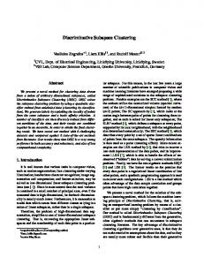
A network made of such layers will be called multilayer kerceptron (MLK). For an illustration of the MLK network, see Fig. 2.1. In MLK, the input (xl ) of each layer is the output of the preceding layer (yl−1 ). The external world is the 0th layer providing input to the first layer of the MLK. l xl = yl−1 ∈ RNI , where NIl is the input dimension of the lth layer. Inputs xl to layer l are mapped by features ϕl and are multiplied by the weights wil . This two-step process can be accomplished implicitly by making use of kernel k l and the expansion property for wil s. The result is vector l sl ∈ RNS , which undergoes nonlinear processing gl , where function gl is differentiable. The output of this nonlinear function is the input to the next layer, i.e., layer xl+1 . The output of the last layer l (layer L, the output of the network) will be referred to as y. Given that yl = xl+1 ∈ RNo , the output l dimension of layer l is No . 2

We assume that the sample space X is the finite dimensional Euclidean space.

19

Hl l

g

...

j

l

i.

...

jl(xl)

yl-1=xl

yl=xl+1

sl

Figure 2.1: The lth layer of the MLK, l = 1, 2, . . . L. The input (xl ) of each layer is the output of the preceding layer (yl−1 ). The external world is the 0th layer providing input to the first layer of the MLK. Inputs xl to layer l are mapped by features mapping ϕl undergo scalar product by the weights (wil ) of the layer in RKHS Hl = Hl (k l ). The result is vector sl , which undergoes nonlinear processing gl , with a differentiable function. The output of this nonlinear function is the input to the next layer, layer xl+1 . The output of the network is the output of the last layer.

2.3.3 Backpropagation of Multilayer Kerceptrons Below, we show that (i) the backpropagation method of MLPs can be extended to MLKs and it (ii) be accomplished in the dual space requiring kernel computations only. We consider a slightly more general task, which incorporates regularizing terms: c(t) = ε2 (t) + r(t) −→

min

{Hl ∋wil : l=1,...,L; i=1,...,NSl }

,

(2.56)

where ε2 (t) = kd(t) − y(t)k22 , NSl

r(t) =

L X X l=1 i=1

(2.57)

2 λli wil (t) Hl

(λli ≥ 0)

(2.58)

are the approximation and the regularization terms of the cost function, respectively, and y(t) denotes the output of the network for the tth input. Parameters λli control the trade-off between approximation and regularization. For λli = 0 the best approximation is searched like in the MLP task [(2.53)]. With these notations at hand, we can present our results [16] now.

 Proposition 2 (explicit case). Let us suppose that the x 7→ w, ϕl (x) Hl and the gl functions are differentiable (l = 1, . . . , L). Then, backpropagation rule can be derived for MLK with cost function (2.56). Proposition 3 (implicit case). Assume that the following holds 1. Constraint on differentiability: Kernels k l are differentiable with respect to both arguments and functions gl are also differentiable (l = 1, . . . , L). 2. Expansion property: The initial weights wil (1) of the network can be expressed in the dual representation, i.e., Nil (1) l

H ∋

wil (1)

=

X

αli,j (1)ϕl (zli,j (1))

j=1

20

(l = 1, . . . , L; i = 1, . . . , NSl ).

(2.59)

Then backpropagation can be derived for MLK with cost function (2.56). This procedure preserves the expansion property (2.59), which then remains valid for the tuned network. The algorithm is implicit in the sense that it can be realized in the dual space, using kernel computations only. The pseudocodes of the MLK backpropagation algorithms are provided in Table 2.5 and Table 2.6, respectively. The MLK backpropagation can be envisioned as follows (see Table 2.5 and 2.6 simultaneously): 1. backpropagated error δ l (t) starts from δ L (t) and is computed by a backward recursion via the l+1 (t)] . differential expression ∂[s ∂[sl (t)] l+1

(t)] can be determined by means of feature mapping ϕl+1 , or, in an implicit 2. expression ∂[s ∂[sl (t)] fashion, through kernels k l+1 .

3. two components play roles in the tuning of w-s: (a) forgetting is accomplished by scaling the weights wil with multiplier 1 − 2µli (t)λli , where λli is the regularization coefficient. (b) adaptation occurs through the backpropagated error. Weights at layer l are tuned by feature space representation of xl (t), the actual input arriving at layer l. Tuning is weighted by the backpropagated error. Derivations of these algorithms are provided in Appendix A.3.

21

Table 2.5: Pseudocode of the explicit MLK backpropagation algorithm. Inputs sample points: {x(t), d(t)}t=1,...,T ,T cost function: λli ≥ 0 (l = 1, . . . , L; i = 1, . . . , NSl ) learning rates: µli (t) > 0 (l = 1, . . . , L; i = 1, . . . , NSl ; t = 1, . . . , T ) Network initialization size: L (number of layers), NIl , NSl , Nol (l = 1, . . . , L) parameters: wil (1) (l = 1, . . . , L; i = 1, . . . , NSl ) Start computation Choose sample x(t) Feedforward computation xl (t) (l = 2, . . . , L + 1), sl (t) (l = 2, . . . , L)a Error backpropagation l=L while l ≥ 1 if (l = L)
′ δ L (t) = 2 [y(t) − d(t)]T gL (sL (t)) else   .. .    ∂ [hwil+1 (t),ϕl+1 (u)iHl+1 ]  l
′ l ∂[sl+1 (t)]   g (s (t))b = ∂[u]  ∂[sl (t)] u=xl+1 (t)   .. . l+1

(t)] δ l (t) = δ l+1 (t) ∂[s ∂[sl (t)]

end Weight update for all i: 1 ≤ i ≤ NSl wil (t + 1) = (1 − 2µli (t)λli )wil (t) − µli (t)δil (t)ϕl (xl (t)) l =l−1 End computation a b

The output of the network, i.e., y(t) = xL+1 (t) is also computed. Here: i = 1, . . . , NSl+1 .

22

Table 2.6: Pseudocode of the implicit MLK backpropagation algorithm. Inputs sample points: {x(t), d(t)}t=1,...,T ,T cost function: λli ≥ 0 (l = 1, . . . , L; i = 1, . . . , NSl ) learning rates: µli (t) > 0 (l = 1, . . . , L; i = 1, . . . , NSl ; t = 1, . . . , T ) Network initialization size: L (number of layers), NIl , NSl , Nol (l = 1, . . . , L) parameters: wil (1)-expansions (l = 1, . . . , L; i = 1, . . . , NSl ) l coefficients: αli (1) ∈ RNi (1) ancestors: zli,j (1), where j = 1, . . . , Nil (1) Start computation Choose sample x(t) Feedforward computation xl (t) (l = 2, . . . , L + 1), sl (t) (l = 2, . . . , L)a Error backpropagation l=L while l ≥ 1 if (l = L)
′ δ L (t) = 2 [y(t) − d(t)]T gL (sL (t)) else   .. .   l+1   Ni (t)
′ l+1   P ∂[s (t)] l+1 l+1 l+1 ′ l+1 =  αij (t)[k ]y (zij (t), x (t))  gl (sl (t))b ∂[sl (t)]   j=1   .. . ∂[sl+1 (t)] l l+1 δ (t) = δ (t) ∂[sl (t)] end Weight update for all i: 1 ≤ i ≤ NSl Nil (t + 1) = Nil (t) + 1
 αli (t + 1) = 1 − 2µli (t)λli αli (t); −µli (t)δil (t) zli,j (t + 1) = zli,j (t) (j = 1, . . . , Nil (t)) zli,j (t + 1) = xl (t) (j = Nil (t + 1)) l =l−1 End computation a b

The output of the network, i.e., y(t) = xL+1 (t) is also computed. i = 1, . . . , NSl+1 . Note also that (k l )′y denotes the derivative of kernel k l according to its second argument.

23

Chapter 3

Theory – Independent Subspace Based Dictionary Learning In this chapter we present our novel independent subspace based dictionary learning approaches. Contrary to Chapter 2, where the underlying assumption for the hidden sources was sparsity and structured sparsity, here we are dealing with indepedent non-Gaussian sources. In Section 3.1 we unify contolled dynamical systems and independent subspace based dictionary learning. Section 3.2 is about the extension of the current ISA models to the partially observable case. In Section 3.3 and Section 3.4 we are dealing with complex and nonparametric generalizations, respectively. Section 3.5 is devoted to the convolutive case. We note that the different methods can be used in combinations, too. For all the introduced models, we derive separation principle based solution. These separation principles make it possible to estimate the models even in case of different, or unknown dimensional independent source components. In Section 3.6 we present a novel random projection based, parallel estimation technique for high dimensional information theoretical quantities. Numerical experiments demonstrating the efficiency of our methods are given in Chapter 5.

3.1 Controlled Models The traditional ICA/ISA problem family can model hidden independent variables, but does not allow/handle control variables. In this section we couple ISA based dictionary learning methods with control variables. To emphasize the fact that we are dealing with sources having dynamics, in the sequel, we will refer to such problems as independent process analysis (IPA)–instead of ISA. In our approach will adapt the D-optimal identification of ARX (autoregressive with exogenous input) dynamical systems, that we briefly summarize in Section 3.1.1. Section 3.1.2 defines the problem domain, the ARX-IPA task. Our solution technique for the ARX-IPA problem is derived in Section 3.1.3.

3.1.1 D-optimal Identification of ARX Models We sketch the basic thoughts that lead to D-optimal identification of ARX models. The dynamical system to be identified is fully observed and evolves according to the ARX equation st+1 =

LX s −1 i=0

Fi st−i +

LX u −1 j=0

24

Bj ut+1−j + et+1 ,

(3.1)

where (i) s ∈ RDs , e ∈ RDe (Ds = De ) represent the state of the system and the noise, respectively, (ii) u ∈ RDu represents the control variables, and (iii) polynomial matrix (given by matrices Fi ∈ RDs ×Ds and identity matrix I) F[z] = I −

LX s −1 i=0

Fi z i+1 ∈ R[z]Ds ×Ds

(3.2)

is stable, that is det(F[z]) 6= 0,

(3.3)

for all z ∈ C, |z| ≤ 1. Our task is (i) the efficient estimation of parameters Θ = [F0 , . . . , FLs −1 , B0 , . . . , BLu −1 ] that determine the dynamics and (ii) noise e that drives the process by the ‘optimal choice’ of control values u. Formally, the aim of D-optimality is to maximize one of the two objectives Jpar (ut+1 ) = I(Θ, st+1 |st , st−1 , . . . , ut+1 , ut , . . .),

Jnoise (ut+1 ) = I(et+1 , st+1 |st , st−1 , . . . , ut+1 , ut , . . .)

(3.4) (3.5)

for ut+1 ∈ U . In other words, we choose control value u from the achievable domain U (e.g., from a box domain) such that it maximizes the mutual information between the next observation and the parameters (or the driving noise) of the system. It can be shown [208], that if (i) Θ has matrix Gaussian, (ii) e has Gaussian, and the covariance matrix of e has inverted Wishart distribution, then in the Bayesian setting, maximization of the J objectives can be reduced to the solution of a quadratic programming task, priors of Θ and e remain in their supposed distribution family and undergo simple updating. The considerations allow for control, but assume full observability about the state variables. Now, we extend the method to hidden variables in the ARX-IPA model of the next section.

3.1.2 The ARX-IPA Problem In the ARX-IPA model we assume that state s of the system cannot be observed directly, but its linear and unknown mixture (x) is available for observation [10]: st+1 =

LX s −1 i=0

xt = Ast ,

Fi st−i +

LX u −1

Bj ut+1−j + et+1 ,

(3.6)

j=0

(3.7)

where Ls and Lu denote the number of the Fi ∈ RDs ×Ds , Bj ∈ RDs ×Du matrices in the corresponding sums. We assume PM • for the em ∈ Rdm components of e = [e1 ; . . . ; eM ] ∈ RDs (Ds = m=1 dm ) that at most one of them may be Gaussian, their temporal evolution is i.i.d. (independent identically distributed), and I(e1 ; . . . ; eM ) = 0; that is, they satisfy the ISA assumptions.1 PLs −1 Fi z i+1 is stable and the mixing matrix A ∈ • that the polynomial matrix F[z] = I − i=0 Ds ×Ds is invertible. We note, that compared to Chapter 2, in the presented ISA based models R the mixing matrix A plays the role of the dictionary. 1 By d -dimensional em components, we mean that em s cannot be decomposed into smaller dimensional independent m parts. This property is called irreducibility in [242].

25

Ls −1 u −1 The ARX-IPA task is to estimate the unknown mixing matrix A, parameters {Fi }i=0 , {Bj }L j=0 , s and e by means of observations x only. In the special case of Ls = Lu = 0, that is

x = Ae

(3.8)

we get back the traditional ISA problem, where the goal is estimate the mixing matrix A and the hidden source e, and there is no control. If dm = 1 (∀m) also holds in ISA, i.e., the independent em source components are one-dimensional, we obtain the ICA problem.

3.1.3 Identification Method for ARX-IPA Below, we solve the ARX-IPA model, i.e., we include the control variables in IPA. We derive a separation principle based solution by transforming the estimation into two subproblems: to that of a fully observed model (Section 3.1.1) and an ISA task. One can apply the basis transformation rule of ARX processes and use (3.6) and (3.7) repeatedly to get LX LX u −1 s −1 (ABj )ut+1−j + (Aet+1 ). (3.9) (AFi A−1 )xt−i + xt+1 = j=0

i=0

According to the d-dependent central limit theorem [195] the marginals of Aet+1 are approximately Ls −1 u −1 Gaussian and thus the parameters ({AFi A−1 }i=0 , {ABj }L j=0 ) and the noise (Aet+1 ) of process x can be estimated by means of the D-optimality principle that assumes a fully observed process. The estimation of Aet+1 can be seen as the observation of an ISA problem because components em of e are independent. ISA techniques can be used to identify A and then from the estimated parameters of process x, the estimations of Fi and Bj follow. Note: 1. In the above described ARX-IPA technique, the D-optimal ARX procedure is an online estimation for the innovation ε = Ae, the input of the ISA method. To the best of our knowledge, there is no existing online ISA method in the literature. However, having such a procedure, one can easily integrate it into the presented approach to get a fully online ARX-IPA estimation scheme. 2. Similar ideas can be used for the estimation of an ARMAX-IPA [7], or post nonlinear model [11]. In the ARMAX-IPA model, the state equation (3.6) is generalized to Le ≥ 0, i.e., st+1 =

LX s −1 i=0

Fi st−i +

LX u −1

Bj ut+1−j + et+1 +

j=0

LX e −1

Hk et−k .

(3.10)

k=0

PLe In this case, we assume additionally that the polynomial matrix H[z] = I + k=1 Hk z k ∈ Ds ×Ds 2 R[z] is stable. In the PNL ARX-IPA model, the observation equation (3.7) is generalized to xt = f (Ast ), (3.11) where f is an unknown, but component-wise acting invertible mapping. 2 Note

that this requirement is automatically fullfilled for Le = 0, when H[z] = I.

26

3.2 Incompletely Observable Models The goal of this section is to search for independent multidimensional processes subject to missing and mixed observations. In spite of the popularity of ICA and its numerous successful applications, the case of missing observation has been considered only for the simplest ICA model in the literature [219, 220]. In this section we extend the solution to (i) multidimensional sources (ISA) and (ii) ease the i.i.d. constraint; we consider AR processes, the AR independent process analysis (AR-IPA) problem.

3.2.1 The AR-IPA Model with Missing Observations We define the AR-IPA model for missing observations (mAR-IPA) [4, 5]. Let us assume that we can only partially (at certain coordinates/time instants) observe (y) the mixture (x) of independent AR sources, that is st+1 =

LX s −1

Fl st−l + et+1 ,

xt = Ast ,

yt = Mt (xt ),

(3.12)

l=0

where • the driving noises, or the innovations em ∈ Rdm (e = [e1 ; . . . ; eM ] ∈ RD ) of the hidden PM source s ∈ RD (D = m=1 dm ) are independent, at least one of them is Gaussian, and i.i.d. in time, i.e., they satisfy the ISA assumptions. • the unknown mixing matrix A ∈ RD×D is invertible, PLs −1 Fl z l+1 ∈ R[z]D×D is stable and • the AR dynamics F[z] = I − l=0

• the Mt ‘mask mappings’ represent the coordinates and the time indices of the non-missing observations.

Our task is the estimation of the hidden source s and the mixing matrix A (or its inverse W) from observation y. For the special choice of Mt = identity (∀t), the AR-IPA problem [173] is obtained. If Ls = 0 also hold, we get the ISA task.

3.2.2 Identification Method for mAR-IPA The mAR-IPA identification can be accomplished as follows. Observation xt is invertible linear transformation of the hidden AR process s and thus it is also an AR process with innovation Aet+1 : xt+1 =

LX s −1

AFl A−1 xt−l + Aet+1 .

(3.13)

l=0

According to the d-dependent central limit theorem [195], the marginals of variable Ae are approximately Gaussian, so one carry out the estimation by 1. identifying the partially observed AR process yt , and then by 2. estimating the independent components em from the estimated innovation by means of ISA.

27

3.3 Complex Models Current methods in the ICA literature are only capable of coping with one-dimensional complex indepedent sources, i.e., with the simplest ICA model. In this section by extending the independent subspace analysis model to complex variables, we make it possible the tackle problems with multidimensinal independent sources. First we summarize a few basic concepts for complex random variables (Section 3.3.1). In Section 3.3.2 the complex ISA model is introduced. In Section 3.3.3 we show, that under certain non-Gaussian assumptions the solution of the complex ISA problem can be reduced to the solution of a real ISA problem.

3.3.1 Complex Random Variables Below we summarize a few basic concept of complex random variables, define two mappings that will be useful in the next section and note that an excellent review on this topic can be found in [172]. A complex random variable v ∈ CL is defined as a random variable of the form v = vR + ivI ∈ CL , where the real and imaginary parts of v, i.e., vR ∈ RL and vI ∈ RL are real vector random variables. Let us define the ϕv : CL 7→ R2L , ϕM : CL1 ×L2 7→ R2L1 ×2L2 mappings as     ℜ(·) ℜ(·) −ℑ(·) ϕv (v) = v ⊗ , ϕM (M) = M ⊗ , (3.14) ℑ(·) ℑ(·) ℜ(·) where ℜ stands for the real part, ℑ for the imaginary part, subscript ‘v’ (‘M ’) for vector (matrix) and ⊗ is the Kronecker product. Known properties of mappings ϕv , ϕM are as follows [189]: det[ϕM (M)] = | det(M)|2

(M ∈ CL×L ), (M1 ∈ C

ϕM (M1 M2 ) = ϕM (M1 )ϕM (M2 ) ϕv (Mv) = ϕM (M)ϕv (v)

(M ∈ C

L1 ×L2

(M ∈ C

L1 ×L2

(M1 , M2 ∈ C

ϕM (M1 + M2 ) = ϕM (M1 ) + ϕM (M2 ) ϕM (cM) = cϕM (M)

(3.15)

L1 ×L2

, M2 ∈ C L2

L2 ×L3

, v ∈ C ),

L1 ×L2

),

, c ∈ R).

),

(3.16) (3.17) (3.18) (3.19)

In words: (3.15) describes transformation of determinant, while (3.16), (3.17), (3.18) and (3.19) expresses preservation of operation for matrix-matrix multiplication, matrix-vector multiplication, matrix addition, real scalar-matrix multiplication, respectively. Independence of complex random variables vm ∈ Cdm (m = 1, . . . , M ) is defined as the independence of variables ϕv (vm ), i.e, I(ϕv (v1 ), . . . , ϕv (vM )) = 0,

(3.20)

where I stands for the mutual information and ϕv (vm ) ∈ R2dm (∀m). The entropy of a complex independent variable v ∈ Cd is defined as H(v) = H(ϕv (v)).

(3.21)

3.3.2 Complex Independent Subspace Analysis By the definition of independence for complex random variables detailed above, the complex valued ISA task [17] can be defined alike to the real case [(3.8)] as x = Ae, 28

(3.22)

where A ∈ CD×D is an unknown invertible mixing matrix, the hidden PM source e is i.i.d. in time t and the em ∈ Cdm components of e = [e1 ; . . . ; eM ] ∈ CD (D = m=1 dm ) are independent, i.e., I(ϕv (e1 ), . . . , ϕv (eM )) = 0. The goal is to estimate the mixing matrix A (or its inverse) and the hidden source e by making use of the observations x only.

3.3.3 Identification Method for Complex ISA Now, we show that one can reduce the solution of the complex ISA model to a real ISA problem in case of certain a ‘non-Gaussian’ assumption. Namely, let us in addition assume in the complex ISA model that at most one of the random variables ϕv (em ) ∈ R2dm is Gaussian. Now, applying transformation ϕv to the complex ISA equation (Eq. (3.22)) and making use of the operation preserving properties of transformations ϕv , ϕM [see (3.17)], one gets: ϕv (x) = ϕM (A)ϕv (e).

(3.23)

Given that (i) the independence of em ∈ Cdm is equivalent to that of ϕv (em ) ∈ R2dm , and (ii) the existence of the inverse of ϕM (A) is inherited from A [see (3.15)], we end up with a real valued ISA task with observation ϕv (x) and M pieces of 2dm -dimensional hidden components ϕv (em ). The consideration can also be extended to the non-i.i.d. case, for further details, see [6].

3.4 Nonparametric Models The general ISA problem of separating sources with nonparametric dynamics has been hardly touched in the literature yet [174, 240]. [174] focused on the separation of stationary and ergodic source components of known and equal dimensions in case of constrained mixing matrices. [240] was dealing with wide sense stationary sources that (i) are supposed to be block-decorrelated for all time-shifts and (ii) have equal and known dimensional source components. The goal of this section is to extend ISA to the case of (i) nonparametric, asymptotically stationary source dynamics and (ii) unknown source component dimensions. Particularly, (i) we address the problem of ISA with nonparametric, asymptotically stationary dynamics, (ii) beyond this extension we also treat the case of unknown and possibly different source component dimensions, (iii) we allow the temporal evolution of the sources to be coupled; it is sufficient that their driving noises are independent and (iv) we propose a simple estimation scheme by reducing the solution of the problem to kernel regression and ISA. The structure of this section is as follows: Section 3.4.1 formulates the problem set-up. In Section 3.4.2 we describe our identification method.

3.4.1 Functional Autoregressive Independent Process Analysis In this section we formally define the problem set-up [1]. In our framework we use functional autoregressive (fAR) processes to model nonparametric stochastic time series. Our goal is to develop dual estimation methods, i.e., to estimate both the system parameters and the hidden states for the functional autoregressive independent process analysis (fAR-IPA) model, which is defined as follows. Assume that the observation (x) is a linear mixture (A) of the hidden source (s), which evolves according to an unknown fAR dynamics (f ) with independent driving noises (e). Formally, st = f (st−1 , . . . , st−Ls ) + et ,

(3.24)

xt = Ast ,

(3.25)

29

D×D where the unknown mixing matrix Ls is the order of the process and the  1 A ∈ RM  isDinvertible, PM m dm ∈ R (D = m=1 dm ) satisfy the ISA assumptions. e ∈ R components of e = e ; . . . ; e The goal of the fAR-IPA problem is to estimate (i) the mixing matrix A (or it inverse W = A−1 ), (ii) the original source st and (iii) its driving noise et by using observations xt only. We list a few interesting special cases:

• If we knew the parametric form of f , and if it were linear, then the problem would be the AR-IPA task [173]. • If we assume that the dynamics of the hidden layer is zero-order AR (Ls = 0), then the problem reduces to the original ISA problem [235].

3.4.2 Identification Method for fAR-IPA We consider the dual estimation of the system described in (3.24)–(3.25). In what follows, we will propose a separation technique with which we can reduce the fAR-IPA estimation problem ((3.24)– (3.25)) to a functional AR process identification and an ISA problem. To obtain strongly consistent fAR estimation, the Nadaraya-Watson kernel regression technique is invoked. More formally, the estimation of the fAR-IPA problem (3.24)-(3.25) can be accomplished as follows. The observation process x is invertible linear transformation of the hidden fAR source process st and thus it is also fAR process with innovation Aet xt = Ast = Af (st−1 , . . . , st−Ls ) + Aet −1

= Af (A

−1

xt−1 , . . . , A

(3.26)

xt−Ls ) + Aet = g(xt−1 , . . . , xt−Ls ) + nt ,

(3.27)

where function g(u1 , . . . , uLs ) = Af (A−1 u1 , . . . , A−1 uLs )

(3.28)

describes the temporal evolution of xt , and nt = Aet

(3.29)

stands for the driving noise of the observation. Making use of this form, the fAR-IPA estimation can ˆ t , the estimated innovation of xt . be carried out by fAR fit to observation xt followed by ISA on n Note that Eq. (3.27) can be considered as a nonparametric regression problem; we have ut = [xt−1 , . . . , xt−Ls ],

vt = xt

(t = 1, . . . , T )

(3.30)

samples from the unknown relation vt = g(ut ) + nt ,

(3.31)

where u, v, and n are the explanatory-, response variables and noise, respectively, and g is the unknown conditional mean or regression function. Nonparametric techniques can be applied to estimate the unknown mean function g(U) = E(V|U),

(3.32)

e.g., by carrying out kernel density estimation for random variables (u,v) and u, where E stands for expectation. The resulting Nadaraya-Watson estimator (i) takes the simple form
PT u−ut t=1 vt K h ˆ0 (u) = PT g (3.33)
, u−ut t=1 K h 30

where K and h > 0 denotes the applied kernel (a non-negative real-valued function that integrates to one) and bandwith, respectively. It can be used to provide a strongly consistent estimation of the regression function g for stationary xt processes [203]. It has been shown recently [204] that for first order and only asymptotically stationary fAR processes, under mild regularity conditions, one can get strongly constistent estimation for the innovation nt by applying the recursive version of the Nadaraya-Watson estimator PT βD t vt K(tβ (u − ut )) ˆ (u) = Pt=1 , g T βD K(tβ (u − u )) t t=1 t

(3.34)

where the bandwith is parameterized by β ∈ (0, 1/D).

3.5 Convolutive Models In this section we address the blind subspace deconvolution (BSSD) problem; an the extension of both the blind source deconvolution and the independent subspace analysis tasks. One can think of the BSSD problem as a cocktail party with groups, held in an echoic room. For the undercomplete case, where we have ‘more microphones than sources’, it has been shown recently that the problem can be reduced to ISA by means of temporal concatenation [14]. However, the associated ISA problem can easily become ‘high dimensional’. The dimensionality problem can be circumvented by applying a linear predictive approximation (LPA) based reduction [12]. Here, we show that it is possible to extend the LPA idea to the complete BSSD task, where the number of ‘microphones’ equals to the number of ‘sources’.3 In the undercomplete case, the LPA based solution was based on the observation that the polynomial matrix describing the temporal convolution had, under rather general conditions4, a polynomial matrix left inverse. In the complete case such an inverse doesn’t exist in general. However, provided that the convolution can be represented by an infinite order autoregressive process, one can construct an efficient estimation method for the hidden components via an asymptotically consistent LPA procedure. This thought is used here to extend the technique of [12] to the complete case. The section is structured as follows: in Section 3.5.1 we define the complete blind subspace deconvolution problem, we detail our solution technique in Section 3.5.2.

3.5.1 Complete Blind Subspace Deconvolution Here, we define the BSSD task [14]. Assume that we have M hidden, independent, multidimensional components (random variables). Suppose also that only their xt =

Le X

Hl et−l

(3.35)

l=0

et is the concatenation of convolutive mixture is available for observation, where xt ∈ RDx andP M 1 M De dm (D = , that is e = [e ; . . . ; e ] ∈ R the components em ∈ R e t t t t m=1 dm ). By describing PL e l the convolution using the the polynomial matrix H[z] = l=0 Hl z ∈ R[z]Dx ×De , one may write Eq. (3.35) compactly as x = H[z]e. (3.36) 3 The

overcomplete BSSD task is challenging and as of yet no general solution is known. the coefficients of the undercomplete polynomial matrix are drawn from a non-degenerate continuous distribution, such an inverse exists with probability one [180]. 4 If

31

We assume that the components em fullfill the ISA assumptions. The goal of the BSSD problem is to estimate the original source et by using observations xt only. While Dx > De is the undercomplete case , Dx = De is the complete one. The case Le = 0 corresponds to the ISA task, and if dm = 1 (∀m) also holds, then the ICA task is recovered. In the BSD task dm = 1 (∀m) and Le is a nonnegative integer. Contrary to previous works [12, 14] focusing on the undercomplete BSSD problem, here [9] we address the complete task (D = Dx = De ). In the complete BSSD problem we assume that the polynomial matrix H[z] is stable.

3.5.2 Identification Method for Complete BSSD Below, we derive our separation principle based solution method for the complete BSSD problem. The invertibility of H[z] implies that the observation process x can be represented as an infinite order autoregressive (AR) process [211]: xt =

∞ X

Fj xt−j + F0 et .

(3.37)

j=1

By applying a finite order LPA approximation (fitting an AR process to x), the innovation process F0 et can be estimated. The innovation can be seen as the observation of an ISA problem because components of e are independent: ISA techniques can be used to identify components em . Choosing 1 T →∞ the order of the fitted AR process to x as p = o(T 3 ) −−−−→ ∞, where T denotes the number of samples, guarantees that the AR approximation for the MA (moving average) model is asymptotically consistent [212].

3.6 Information Theoretical Estimations via Random Projections The estimation of relevant information theoretical quantities, such as entropy, mutual information, and various divergences is computationally expensive in high dimensions. However, consistent estimation of these quantities is possible by nearest neighbor (NN) methods (see, e.g., [228]) that use the pairwise distances of sample points. Although search for nearest neighbors can also be expensive in high dimensions [226], low dimensional approximate isometric embedding of points of high dimensional Euclidean space can be addressed by the Johnson-Lindenstrauss Lemma [221] and the related random projection (RP) methods [224, 225]. The RP approach proved to be successful, e.g., in classification, clustering, search for approximate NN (ANN), dimension estimation of manifolds, estimation of mixture of Gaussian models, compressions, data stream computation (see, e.g., [223]). We note that the RP approach is also related to compressed sensing [222]. In this section [8] we show a novel application of the RP technique: we estimate information theoretical quantities using the ANN-preserving properties of the RP technique. We present our RP based approach through the ISA problem. The ISA task can be viewed as the minimization of the mutual information between the estimated components, or equivalently as the minimization of the sum of Shannon’s multidimensional differential entropies of the estimated components on the orthogonal group [239]: M X J(W) = H (ym ) → min , (3.38) W∈O D

m=1

where

y = Wx,

  y = y1 ; . . . ; yM , 32

y m ∈ Rd m

(3.39)

and dm s are given. Estimation of cost function J however involves multidimensional entropy estimation, which is computationally expensive in high dimensions, but can be executed by NN methods consistently [228]. It has been shown in [227] (in the field of image registration with high dimensional features) that the computational load can be decreased somewhat by • dividing the samples into groups and then • computing the averages of the group estimates. We will combine this parallelizable ensemble approach with the ANN-preserving properties of RPs and get drastic savings. We suggest the following entropy estimation method5 , for each estimated m ˆ ISA ISA component v := y : • divide the T samples {v(1), . . . , v(T )} into N groups indexed by sets I1 , . . . , IN so that each group contains K samples, • for all fixed groups take the random projection of v as vn,RP (t) := Rn v(t)

′

(t ∈ In ; n = 1, . . . , N ; Rn ∈ Rdm ×dm ),

(3.40)

• average the estimated entropies of the RP-ed groups to get the estimation N 1 X ˆ ˆ H(vn,RP ). H(v) = N n=1

(3.41)

Our particular choice for Rn can be found in Section 5.3.6.

5 The idea can be used for a number of information theoretical quantities, provided that they can be estimated by means of pairwise Euclidean distances of the samples.

33

Chapter 4

Numerical Experiments – Group-Structured Dictionary Learning In this chapter we demonstrate the efficiency of structured sparse representations. For illustration purposes we chose the online group-structured dictionary learning approach. The efficiency of the method is presented in 3 different applications: inpainting of natural images (Section 4.1), structured non-negative matrix factorization of faces (Section 4.2) and collaborative filtering (Section 4.3).

4.1 Inpainting of Natural Images We studied the following issues on natural images: 1. Is structured dictionary D beneficial for inpainting of patches of natural images, and how does it compare to the dictionary of classical sparse representation? During learning of D, training samples xi were fully observed (i.e., ∆i = I). 2. In this inpainting problem of image patches, we also studied the case when the training samples xi were partially observed (∆i 6= I). 3. We also show results for inpainting of full images using a dictionary learned from partially observed (∆i 6= I) patches. In our numerical experiments we used Di = S2dx (∀i), A = Rdα without additional weighing (A = I, ∀G ∈ G). Group structure G of vector α was realized on a 16 × 16 torus (dα = 256) with |G| = dα applying r = 0, 1, 2, or 3 neighbors to define G. For r = 0 (G = {{1}, . . . , {dα }}) the classical sparse representation is recovered. Our test database was the ICA natural image database.1 We chose 12 of the 13 images of the dataset to study the first two questions above (see Fig. 4.1(a)), and used the 13th picture for studying the third question (Fig. 4.1(b)). For each of the 12 images, we sampled 131, 072 = 217 pieces of 8 × 8 disjunct image patches randomly (without replacement). This patch set was divided to a training set Xtr made of 65, 536 pieces, and to a validation (Xval ) and test ( Xtest ) set with set sizes 32, 768. Each patch was normalized to zero average and unit ℓ2 -norm. G

1 See

http://www.cis.hut.fi/projects/ica/data/images/.

34

(a)

(b)

Figure 4.1: Illustration of the used natural image dataset. (a): 12 images of similar kind were used to select patches for the training Xtr , validation Xval , and test Xtest sets. (b): test image used for the illustration of full image inpainting. In the first experiment xi s were fully observed (∆i = I) and thus the update of their statistics was precise. This is called the BCD case in the figures. Matrix D was learned on the set Xtr , columns dj were initialized by using a uniform distribution on the surface of the ℓ2 -sphere. Pixels of the x patches in the validation and test sets were removed with probability pval test . For a given noise-free image patch x, let xO denote its observed version, where O stands for the indices of the available coordinates. The task was the inpainting of the missing pixels of x by means of the pixels present ( xO ) and by the learned matrix D. After removing the rows of D corresponding to missing pixels of x, the resulting DO and xO were used to estimate α. The final estimation of ˆ = Dα. According to our preliminary experiments, learning rate ρ and mini-batch size x was x R were set to 32 and 64, respectively (the estimation was robust as a function of ρ and R). In the updates of z and α (2.24) only minor changes were experienced after 2-3 iterations, thus the number of iterations Tα was set to 5. Concerning the other parameters, we used η = 0.5, and κ ∈ {2−19 , 2−18 , . . . , 2−10 }. The ǫ smoothing parameter was 10−5 , and the iteration number for the update of D was TD = 5. Values of pval test were chosen from set {0.3, 0.5, 0.7, 0.9}, so for the case of pval test = 0.9, only 10% of the pixels of x were observed. For each fixed neighborhood size r and parameter pval test , κ was chosen as the minimum of mean squared error (MSE) using D trained on patch set Xtr and evaluated on Xval . Having found this optimal κ on the validation set, we used its value to compute the MSE on Xtest . Then we changed the roles of Xval and Xtest , that is, validated on Xtest , and tested on Xval . This procedure was repeated for four random initializations (D0 ) and different corruptions (Xval , Xtest ). The average MSE values (multiplied by 100) and their standard deviations for different neighbor sizes r and corruption rates pval test are summarized in Table 4.1. This table shows that (i) the inpainting error grows with the corruption rate pval test , (ii) compared to sparse representation (r = 0) small neighborhood size r = 1 gives rise to similar results, r = 2 is better and r = 3 seems to be the best for all cases with 13 − 19% improvement in precision for MSE. Learned and average quality dictionaries D can be seen in Fig. 4.2 (r = 0 no structure, r = 2, 3 with torus structure). Based on this experiment we can conclude that the structured algorithm gives rise to better results than ordinary sparse representations. In the second experiment, the size of the neighborhood was fixed, set to r = 3. We learned dictionary D on partially observed patches (∆i 6= I). The probability ptr of missing any pixel from the observations in the training set assumed values from the set {0, 0.1, 0.3, 0.5, 0.7, 0.9}. In this case, we updated e using the approximation Eq. (2.33), hence we call this method approximate-BCD (or BCDA, for short). The other experimental details were identical to the previous case (i.e., when ∆i = I). Results and statistics for MSE are provided for a smaller (0.3) and for a larger (0.7) value of pval test in Table 4.2 for different probability values ptr . We found that increasing ptr up to ptr = 0.7 MSE values grow slowly. Note that we kept the number of samples xi at 65, 536 identical to the previous case (∆i = I), and thus by increasing ptr the effective number of observations/coordinates decreases. Learned average quality dictionaries D are shown in Fig. 4.3 for pval test = 0.7. Note

35

Table 4.1: BCD: 100 × the MSE average (± std) as a function of neighbors (r = 0: sparse representation, no structure) for different pval test corruption rates. pval = 0.3 pval test test = 0.5 r = 0 0.65 (±0.002) 0.83 (±0.003) r = 1 0.60 (±0.005; +6.78%) 0.85 (±0.017; −2.25%) r = 2 0.59 (±0.005; +10.39%) 0.81 (±0.008; +2.67%) r = 3 0.56 (±0.002; +16.38%) 0.71 (±0.002; +16.01%) pval pval test = 0.7 test = 0.9 r = 0 1.10 (±0.002) 1.49 (±0.006) r = 1 1.10 (±0.029; +0.27%) 1.45 (±0.004; +2.96%) r = 2 1.12 (±0.029; −1.09%) 1.46 (±0.029; +2.51%) r = 3 0.93 (±0.001; +18.93%) 1.31 (±0.002; +13.87%) Table 4.2: BCDA (r = 3): 100 × the MSE average (± std) for different pval test and ptr corruption rates. ptr = 0 ptr = 0.1 ptr = 0.3 pval = 0.3 0.55 (±0.003) 0.56 (±0.001) 0.57 (±0.003) test pval = 0.7 0.91 (±0.002) 0.91 (±0.002) 0.91 (±0.002) test ptr = 0.5 ptr = 0.7 ptr = 0.9 pval test = 0.3 0.59 (±0.001) 0.61 (±0.002) 0.71 (±0.007) pval test = 0.7 0.92 (±0.003) 0.93 (±0.002) 0.96 (±0.003) that the MSE values are still relatively small for missing pixel probability ptr = 0.9 (100× MSE maximum is about 0.96), thus our proposed method is still efficient in this case. Reconstruction with value 0.92 (100× MSE) is shown in Fig. 4.4. In our third illustration we show full image inpainting using dictionary D learned with ptr = 0.5 and using the 13th image (X) shown in Fig. 4.1(b). We executed inpainting consecutively on all ˆ i from all 8 × 8 patches of image X and for each pixel of image X, we averaged all estimations x = 0.3 and 0.7 values. 8 × 8 patches that contained the pixel. Results are shown in Fig. 4.4 for pval test We also provide the PSNR (peak signal-to-noise ratio) values of our estimations. This measure for vectors u, v ∈ Rd (i.e., for vectors formed from the pixels of the image) is defined as " # (max(maxi |ui |, maxj |vj |))2 P SN R(u, v) = 10 log10 , (4.1) 2 1 d ku − vk2

(a)

(b)

(c)

Figure 4.2: Illustration of the online learned group-structured D dictionaries with the BCD technique and MSE closest to the average (see Table 4.1) and pval test = 0.7. (a): r = 0, (b): r = 2, (c): r = 3. 36

(a)

(b)

(c)

Figure 4.3: Illustration of the online learned group-structured D dictionaries for the BCDA technique with MSE closest to the average (see Table 4.2) and pval test = 0.7. (a): ptr = 0, (b): ptr = 0.1, (c): ptr = 0.5.

(a)

(b)

(c)

(d)

Figure 4.4: Inpainting illustration using the online learned group-structured D dictionaries for the BCDA technique with MSE closest to the average (see Table 4.2) and ptr = 0.5. (a): measured, (b): val estimated, PSNR = 36 dB. (a)-(b): pval test = 0.3. (c)-(d): the same as (a)-(b), but with ptest = 0.7, in (d) PSNR = 29 dB. where the higher value is the better. Acceptable values in wireless transmission (lossy image and video compression) are around 20 − 25 dB (30 dB). By means of D and for missing probability val pval test = 0.3 we achieved 36 dB PSNR, whereas for missing probability ptest = 0.7 we still have 29 dB PSNR, underlining the efficiency of our method.

4.2 Online Structured Non-negative Matrix Factorization on Faces It has been shown on the CBCL database that dictionary vectors (di ) of the offline NMF method can be interpreted as face components [139]. However, to the best of our knowledge, there is no existing NMF algorithm as of yet, which could handle general G group structures in an online fashion. Our OSDL method is able to do that, can also cope with only partially observed inputs, and can be extended with non-convex sparsity-inducing norms. We illustrate our approach on the color FERET2 dataset: we set Di = S2dx ∩ Rd+x (∀i), A = Rd+α , ∆i = I and η = 0.5. We selected 1, 736 facial 2 See

http://face.nist.gov/colorferet/.

37

Figure 4.5: Illustration of the online learned structured NMF dictionary. Upper left corner: training samples. pictures from the dataset. Using affine transformations we positioned the noses and eyes to the same pixel coordinates, reduced the image sizes to 140 × 120, and set their l2 norms to be one. These images were the observations for our ODSL method (xi , dx = 49, 140 = 140 × 120 × 3 minus some masking). The group structure G was chosen to be hierarchical; we applied a full, 8-level binary tree. Each node with its corresponding descendants formed the sets of G ∈ G (dα = 255). According to our experiments, the learned dictionary D was influenced mostly by the constant κ, and similarly to Section 4.1, it proved to be quite insensitive to the value of the learning factor ρ, and to the size of the mini-batches (R). Fig. 4.5 shows a few elements from the online estimated structured NMF dictionary (using κ = 2−10.5 , ρ = 32, R = 8, AG = I (∀G ∈ G), Tα = 5, TD = 5 and ε = 10−5 ). We can observe that the proposed algorithm is able to naturally develop and hierarchically organize the elements of the dictionary: towards the leaves the learned filters reveal more and more details. We can also notice that the colors are separated as well. This example demonstrates that our method can be used for large problems where the dimension of the observations is about 50, 000.

4.3 Collaborative Filtering The proliferation of online services and the thriving electronic commerce overwhelms us with alternatives in our daily lives. To handle this information overload and to help users in efficient decision making, recommender systems (RS) have been designed. The goal of RSs is to recommend personalized items for online users when they need to choose among several items. Typical problems include recommendations for which movie to watch, which jokes/books/news to read, which hotel to stay at, or which songs to listen to. One of the most popular approaches in the field of recommender systems is collaborative filtering (CF). The underlying idea of CF is very simple: Users generally express their tastes in an explicit way by rating the items. CF tries to estimate the users’ preferences based on the ratings they have already made on items and based on the ratings of other, similar users. For a recent review on recommender systems and collaborative filtering, see e.g., [158].

38

Novel advances on CF show that dictionary learning based approaches can be efficient for making predictions about users’ preferences [160]. The dictionary learning based approach assumes that (i) there is a latent, unstructured feature space (hidden representation) behind the users’ ratings, and (ii) a rating of an item is equal to the product of the item and the user’s feature. To increase the generalization capability, usually ℓ2 regularization is introduced both for the dictionary and for the users’ representation. Here, we extend the application domain of structured dictionary learning in the direction of collaborative filtering. With respect to CF, further constraints appear for structured dictonary learning since (i) online learning is desired and (ii) missing information is typical. There are good reasons for them: novel items/users may appear and user preferences may change over time. Adaptation to users also motivate online methods. Furthermore, users can evaluate only a small portion of the available items, which leads to incomplete observations, missing rating values. To do so, we formulate the CF task as an OSDL optimization problem in Section 4.3.1. According to the CF literature, oftentimes neighbor-based corrections improve the precision of the estimation. We also use this technique (Section 4.3.2) to improve the OSDL estimations. Numerical results are presented in Section 4.3.3.

4.3.1 Collaborative Filtering as Structured Dictionary Learning Below, the CF task is transformed into an OSDL problem. Consider the tth user’s known ratings as OSDL observations xOt . Let the optimized group-structured dictionary on these observations be D. Now, assume that we have a test user and his/her ratings, i.e., xO ∈ R|O| . The task is to estimate x{1,...,dx }\O , that is, the missing coordinates of x (the missing ratings of the user) that can be accomplished as follows: 1. Remove the rows of the non-observed {1, . . . , dx }\O coordinates from D. The obtained |O| × dα sized matrix DO and xO can be used to estimate α by solving the structured sparse coding problem (2.2). 2. Using the estimated representation α, estimate x as ˆ = Dα. x

(4.2)

4.3.2 Neighbor Based Correction According to the CF literature, neighbor based correction schemes may further improve the precision of the estimations [158]. This neighbor correction approach • relies on the assumption that similar items (e.g., jokes/movies) are rated similarly and • it can be adapted to OSDL-based CF estimation in a natural fashion. Here, we detail the idea. Let us assume that the similarities sij ∈ R (i, j ∈ {1, . . . , dx }) between individual items are given. We shall provide similarity forms in Section 4.3.3. Let dk αt ∈ R be the OSDL estimation for the rating of the k th non-observed item of the tth user (k 6∈ Ot ), where dk ∈ R1×dα is the k th row of matrix D ∈ Rdx ×dα , and αt ∈ Rdα is computed according to Section 4.3.1. Let the prediction error on the observable item neighbors (j) of the k th item of the tth user (j ∈ Ot \{k}) be dj αt − xjt ∈ R. These prediction errors can be used for the correction of the

39

OSDL estimation (dk αt ) by taking into account the sij similarities: "P # j j∈Ot \{k} skj (d αt − xjt ) k P xˆkt = d αt + γ1 , or j∈Ot \{k} skj # "P j s (d α − x ) kj t jt j∈O \{k} t P , xˆkt = γ0 (dk αt ) + γ1 j∈Ot \{k} skj

(4.3)

(4.4)

where k 6∈ Ot . Here, (4.3) is analogous to the form of [160], (4.4) is a simple modification: it modulates the first term with a separate γ0 weight.

4.3.3 Numerical Results This section is structured as follows: We have chosen the Jester dataset for the illustration of the OSDL based CF approach. It is a standard benchmark for CF. This is what we introduce first. Then we present our preferred item similarities. The performance measure used to evaluate the CF based estimation follows. The final part of this section is about our numerical experiences. The Jester Dataset The dataset [161] contains 4, 136, 360 ratings from 73, 421 users to 100 jokes on a continuous [−10, 10] range. The worst and best possible gradings are −10 and +10, respectively. A fixed 10 element subset of the jokes is called gauge set and it was evaluated by all users. Two third of the users have rated at least 36 jokes, and the remaining ones have rated between 15 and 35 jokes. The average number of user ratings per joke is 46. Item Similarities In the neighbor correction step (4.3) or (4.4) we need the sij values representing the similarities of the ith and j th items. We define this value as the similarity of the ith and j th rows (di and dj ) of the optimized OSDL dictionary D [160]:

 !β max(0, di , dj ) i j S1 : sij = sij (d , d ) = , or (4.5) kdi k2 kdj k2

i

!−β

d − dj 2 2 , (4.6) S2 : sij = sij (di , dj ) = kdi k2 kdj k2 where β > 0 is the parameter of the similarity measure. Quantities sij are non-negative; if the value of sij is close to zero (large) then the ith and j th items are very different (very similar). Performance Measure In our numerical experiments we used the RMSE (root mean square error) measure for the evaluation of the quality of the estimation, since RMSE is one of most popular measures in the CF literature. The RMSE measure is the average squared difference of the true and the estimated rating values: v u u 1 X (xit − x ˆit )2 , (4.7) RM SE = t |S| (i,t)∈S

where S denotes either the validation or the test set. 40

Evaluation Here we illustrate the efficiency of the OSDL-based CF estimation on the Jester database using the RMSE performance measure. To the best of our knowledge, the top results on this database are RMSE = 4.1123 [159] and RMSE = 4.1229 [160]. Both works are from the same authors. The method in the first paper is called item neigbor and it makes use of only neighbor information. In [160], the authors used a bridge regression based unstructured dictionary learning model—with a neighbor correction scheme—, they optimized the dictionary by gradient descent and set dα to 100. These are our performance baselines. To study the capability of the OSDL approach in CF, we focused on the following issues: • Is structured dictionary D beneficial for prediction purposes, and how does it compare to the dictionary of classical (unstructured) sparse dictionary? • How does the OSDL parameters and the similarity/neighbor correction applied affect the efficiency of the prediction? • How do different group structures G fit to the CF task?

In our numerical studies we chose the Euclidean unit sphere for Di = S2dx (∀i), and A = Rdα , and no additional weighing was applied (dG = χG , ∀G ∈ G, where χ is the indicator function). We set η of the group-structured regularizer Ω to 0.5. Group structure G of vector α was realized on • a d × d toroid (dα = d2 ) with |G| = dα applying r ≥ 0 neighbors to define G. For r = 0 (G = {{1}, . . . , {dα }}) the classical sparse representation based dictionary is recovered. • a hierarchy with a complete binary tree structure. In this case: – |G| = dα , and group G of αi contains the ith node and its descendants on the tree, and

– the size of the tree is determined by the number of levels l. The dimension of the hidden representation is then dα = 2l − 1. The size R of mini-batches was set either to 8, or to 16 and the forgetting rate ρ was chosen from 1 1 1 1 1 1 , 32 , 16 , 8 , 4 , 2 , 1}. The κ weight of structure inducing regularizer Ω was chosen from set {0, 64 1 1 the set { 2−1 , 20 , 211 , 212 , 214 , 216 , . . . , 2114 }. We studied similarities S1 , S2 [see (4.5)-(4.6)] with both neighbor correction schemes [(4.3)-(4.4)]. In what follows, corrections based on (4.3) and (4.4) will be called S1 , S2 and S10 , S20 , respectively. Similarity parameter β was chosen from the set {0.2, 1, 1.8, 2.6, . . . , 14.6}. In the BCD step of the optimization of D, Tα = 5 iterations were applied. In the α optimization step, we used TD = 5 iterations, whereas smoothing parameter ǫ was 10−5 . We used a 90% − 10% random split for the observable ratings in our experiments, similarly to [160]: • training set (90%) was further divided into 2 parts: – we chose the 80% observation set {Ot } randomly, and optimized D according to the corresponding xOt observations, – we used the remaining 10% for validation, that is for choosing the optimal OSDL parameters (r or l, κ, ρ), BCD optimization parameter (R), neighbor correction (S1 , S2 , S10 , S20 ), similarity parameter (β), and correction weights (γi s in (4.3) or (4.4)). • we used the remaining 10% of the data for testing. The optimal parameters were estimated on the validation set, and then used on the test set. The resulting RMSE score was the performance of the estimation. 41

Toroid Group Structure. In this section we provide results using toroid group structure. We set d = 10. The size of the toroid was 10 × 10, and thus the dimension of the representation was dα = 100. In the first experiment we study how the size of neighborhood (r) affects the results. This parameter corresponds to the ‘smoothness’ imposed on the group structure: when r = 0, then there is no relation between the dj columns in D (no structure). As we increase r, the dj feature vectors will be more and more aligned in a smooth way. To this end, we set the neighborhood size to r = 0 (no structure), and then increased it to 1, 2, 3, 4, and 5. For each (κ, ρ, β), we calculated the RMSE of our estimation, and then for each fixed (κ, ρ) pair, we minimized these RMSE values in β. The resulting validation and test surfaces are shown in Fig. 4.6. For the best (κ, ρ) pair, we also present the RMSE values as a function of β (Fig. 4.7). In this illustration we used S10 neighbor correction and R = 8 mini-batch size. We note that we got similar results using R = 16 too. Our results can be summarized as follows. • For a fixed neighborhood parameter r, we have that: – The validation and test surfaces are very similar (see Fig. 4.6(e)-(f)). It implies that the validation surfaces are good indicators for the test errors. For the best r, κ and ρ parameters, we can observe that the validation and test curves (as functions of β) are very similar. This is demonstrated in Fig. 4.7, where we used r = 4 neighborhood size and S10 neighbor correction. We can also notice that (i) both curves have only one local minimum, and (ii) these minimum points are close to each other. – The quality of the estimation depends mostly on the κ regularization parameter. As we increase r, the best κ value is decreasing. – The estimation is robust to the different choices of forgetting factors (see Fig. 4.6(a)-(e)). In other words, this parameter ρ can help in fine-tuning the results. • Structured dictionaries (r > 0) are advantageous over those methods that do not impose structure on the dictionary elements (r = 0). For S10 and S20 neighbor corrections, we summarize the RMSE results in Table 4.3. Based on this table we can conclude that in the studied parameter domain – the estimation is robust to the selection of the mini-batch size (R). We got the best results using R = 8. Similarly to the role of parameter ρ, adjusting R can be used for fine-tuning. – the S10 neighbor correction lead to the smallest RMSE value. – When we increase r up to r = 4, the results improve. However, for r = 5, the RMSE values do not improve anymore; they are about the same that we have using r = 4. – The smallest RMSE we could achieve was 4.0774, and the best known result so far was RMSE = 4.1123 [159]. This proves the efficiency of our OSDL based collaborative filtering algorithm. – We note that our RMSE result seems to be significantly better than the that of the competitors: we repeated this experiment 5 more times with different randomly selected training, test, and validation sets, and our RMSE results have never been worse than 4.08. In the second experiment we studied how the different neighbor corrections (S1 , S2 , S10 , S20 ) affect the performance of the proposed algorithm. To this end, we set the neighborhood parameter to r = 4 because it proved to be optimal in the previous experiment. Our results are summarized in Table 4.4. From these results we can observe that 42

r=0

r=1

2

8

4.23

4.3 Regularization (−log2(κ))

Regularization (−log2(κ))

4.22 4.21 1 4.2 4.19 4.18

0

4.17

4.28 4.26

6

4.24 4.22 4.2 4

4.18 4.16

4.16

4.14

−1 0

4.15 1/64 1/32 1/16 1/8 1/4 Learning rate (ρ)

1/2

2 0

1

(a)

14

4.18

4.095

4.17

Regularization (−log2(κ))

Regularization (−log2(κ))

1

r=3

r=2

4.16

10

4.15 4.14

8

4.13 4.12 1/64 1/32 1/16 1/8 1/4 Learning rate (ρ)

1/2

(b)

12

6 0

1/64 1/32 1/16 1/8 1/4 Learning rate (ρ)

1/2

4.085 4.08

10

4.075 8 0

1

4.09

12

(c)

1/64 1/32 1/16 1/8 1/4 Learning rate (ρ)

1/2

1

(d)

r=4

r=4

14

14 4.14 Regularization (−log2(κ))

4.13

2

Regularization (−log (κ))

4.14

12

4.12 4.11 4.1

10 4.09

4.13 12

4.12 4.11 4.1

10 4.09

4.08 8 0

4.07

1/64 1/32 1/16 1/8 1/4 Learning rate (ρ)

1/2

1

4.08

4.07

8 0

(e)

1/64 1/32 1/16 1/8 1/4 Learning rate (ρ)

1/2

1

4.07

(f)

Figure 4.6: Validation surfaces [(a)-(e)] and test surfaces (f) as a function of forgetting factor (ρ) and regularization (κ). For a fixed (κ, ρ) parameter pair, the surfaces show the best RMSE values optimized in the β similarity parameter. The group structure (G) is toroid. The applied neighbor correction was S10 . (a): r = 0 (no structure). (b): r = 1. (c): r = 2. (d): r = 3. (e)-(f): r = 4, on the same scale.

43

4.11 Validation curve Test curve

RMSE

4.1 4.09 4.08 4.07

0

5 10 Similarity parameter (β)

15

Figure 4.7: Validation and test curves for toroid group structure using the optimal neighborhood size r = 4, regularization weight κ = 2110 , forgetting factor ρ = 215 , mini-batch size R = 8, and similarity parameter β = 3.4. The applied neighbor correction was S10 . Table 4.3: Performance (RMSE) of the OSDL prediction using toroid group structure (G) with different neighbor sizes r (r = 0: unstructured case). First-second row: mini-batch size R = 8, third-fourth row: R = 16. Odd rows: S10 , even rows: S20 neighbor correction. For fixed R, the best performance is highlighted with boldface typesetting. r=0 r=1 r=2 r=3 r=4 0 R = 8 S1 4.1594 4.1326 4.1274 4.0792 4.0774 S20 4.1765 4.1496 4.1374 4.0815 4.0802 R = 16 S10 4.1611 4.1321 4.1255 4.0804 4.0777 S20 4.1797 4.1487 4.1367 4.0826 4.0802 • our method is robust to the selection of correction methods. Similarly to the ρ and R parameters, the neighbor correction parameter can help in fine-tuning the results. • The introduction of γ0 in (4.4) with the application of S10 and S20 instead of S1 and S2 proved to be advantageous in the neighbor correction phase. • For the studied CF problem, the S10 neighbor correction method (with R = 8) lead to the smallest RMSE value, 4.0774. • The R ∈ {8, 16} setting yielded us similarly good results. Even with R = 16, the RMSE value was 4.0777.

Table 4.4: Performance (RMSE) of the OSDL prediction for different neighbor corrections using toroid group structure (G). Columns: applied neighbor corrections. Rows: mini-batch size R = 8 and 16. The neighbor size was set to r = 4. For fixed R, the best performance is highlighted with boldface typesetting. S1 S2 S10 S20 R = 8 4.0805 4.0844 4.0774 4.0802 R = 16 4.0809 4.0843 4.0777 4.0802

44

Hierarchical Group Structure. In this section we provide results using hierarchical α representation. The group structure G was chosen to represent a complete binary tree. In our third experiment we study how the number of levels (l) of the tree affects the results. To this end, we set the number of levels to l = 3, 4, 5, and 6. Since dα , the dimension of the hidden representation α, equals to 2l − 1, these l values give rise to dimensions dα = 7, 15, 31, and 63. Validation and test surfaces are provided in Fig. 4.8(a)-(c) and (e)-(f), respectively. The surfaces show for each (κ, ρ) pair, the minimum RMSE values taken in the similarity parameter β. For the best (κ, ρ) parameter pair, the dependence of RMSE on β is presented in Fig. 4.8(d). In this illustration we used S10 neighbor correction, and the mini-batch size was set to R = 8. Our results are summarized below. We note that we obtained similar results with mini-batch size R = 16. • For fixed number of levels l, similarly to the toroid group structure (where the size r of the neighborhood was fixed), – validation and test surfaces are very similar, see Fig. 4.8(b)-(c). Validation and test curves as a function of β behave alike, see Fig. 4.8(d). – the precision of the estimation depends mostly on the regularization parameter κ; forgetting factor ρ enables fine-tuning. • The obtained RMSE values are summarized in Table 4.5 for S10 and S20 neighbor corrections. According to the table, the quality of estimation is about the same for mini-batch size R = 8 and R = 16; the R = 8 based estimation seems somewhat more precise. Considering the neighbor correction schemes S10 and S20 , S10 provided better predictions. • As a function of the number of levels, we got the best result for l = 4, RMSE = 4.1220; RMSE values decrease until l = 4 and then increase for l > 4. • Our best obtained RMSE value is 4.1220; it was achieved for dimension only dα = 15. We note that this small dimensional, hierarchical group structure based result is also better than that of [160] with RMSE = 4.1229, which makes use of unstructured dictionaries with dα = 100. The result is also competitive with the RMSE = 4.1123 value of [159]. In our fourth experiment we investigate how the different neighbor corrections (S1 , S2 , S10 , S20 ) affect the precision of the estimations. We fixed the number of levels to l = 4, since it proved to be the optimal choice in our previous experiment. Our results are summarized in Table 4.6. We found that • the estimation is robust to the choice of neighbor corrections, • it is worth including weight γ0 [see (4.4)] to improve the precision of prediction, that is, to apply correction S10 and S20 instead of S1 and S2 , respectively. • the studied R ∈ {8, 16} mini-batch sizes provided similarly good results. • for the studied CF problem the best RMSE value was achieved using S10 neighbor correction and mini-batch size R = 8.

45

l=3

l=4

4

4

Regularization (−log2(κ))

4.24

2

Regularization (−log (κ))

4.25

2 4.2 1

0 0

4.15 1/64 1/32 1/16 1/8 1/4 Learning rate (ρ)

1/2

4.22 2

4.2 4.18 4.16

1

4.14 0 0

1

4.12 1/64 1/32 1/16 1/8 1/4 Learning rate (ρ)

(a)

1/2

1

(b)

l=4 4.24

4.16

4.22

4.15

2

Regularization (−log (κ))

4

2

RMSE

4.2 4.18

Validation curve Test curve

4.14 4.13

4.16

1

4.12 4.14 0 0

4.11 0

4.12 1/64 1/32 1/16 1/8 1/4 Learning rate (ρ)

1/2

1

5 10 Similarity parameter (β)

(c)

15

(d) l=6

l=5

6

6

4.45

Regularization (−log2(κ))

4.4

2

Regularization (−log (κ))

4.45

4

4.35 4.3 4.25

2

4.2

4.4 4

4.35 4.3 4.25

2

4.2

4.15 1 0

1/64 1/32 1/16 1/8 1/4 Learning rate (ρ)

1/2

4.15 1 0

1

(e)

1/64 1/32 1/16 1/8 1/4 Learning rate (ρ)

1/2

1

(f)

Figure 4.8: Validation surfaces [(a)-(b), (e)-(f)] and test surfaces (c) as a function of forgetting factor (ρ) and regularization (κ). (d): validation and test curve using the optimal number of levels l = 4, regularization weight κ = 212 , forgetting factor ρ = 0, mini-bach size R = 8, similarity parameter β = 1.8. Group structure (G): complete binary tree. Neighbor correction: S10 . (a)-(c),(e)-(f): for fixed (κ, ρ) parameter pair, the surfaces show the best RMSE values optimized in the β similarity parameter. (a): l = 3. (b)-(c): l = 4, on the same scale. (e): l = 5. (f): l = 6.

46

Table 4.5: Performance (RMSE) of the OSDL prediction for different number of levels (l) using binary tree structure (G). First-second row: mini-batch size R = 8, third-fourth row: R = 16. Odd rows: S10 , even rows: S20 neighbor correction. For fixed R, the best performance is highlighted with boldface typesetting. l=3 l=4 l=5 l=6 R = 8 S10 4.1572 4.1220 4.1241 4.1374 S20 4.1669 4.1285 4.1298 4.1362 R = 16 S10 4.1578 4.1261 4.1249 4.1373 S20 4.1638 4.1332 4.1303 4.1383

Table 4.6: Performance (RMSE) of the OSDL prediction for different neighbor corrections using binary tree structure (G). Rows: mini-batch size R = 8 and 16. Columns: neighbor corrections. Neighbor size: r = 4. For fixed R, the best performance is highlighted with boldface typesetting. S1 S2 S10 S20 R = 8 4.1255 4.1338 4.1220 4.1285 R = 16 4.1296 4.1378 4.1261 4.1332

47

Chapter 5

Numerical Experiments – Indepedent Subspace Based Dictionary Learning In this chapter we illustrate the efficiency of the proposed IPA estimation methods (Chapter 3). Test databases are described in Section 5.1. To evaluate the solutions, we use the performance measure given in Section 5.2. Our numerical results are presented in Section 5.3.

5.1 Test Datasets We conducted experiments using the following datasets to assess the efficiency and robustness of our methods: ABC, 3D-geom: In the ABC database, the distribution of the hidden sources em were uniform on 2-dimensional images (dm = 2) of the English alphabet. The number of components can be M = 26. For illustration, see Fig. 5.1(b). In the 3D-geom test em s were random variables uniformly distributed on 3-dimensional geometric forms (dm = 3, M = 6), see Fig. 5.1(a). celebrities, smiley: The celebrities and smiley test has 2-dimensional source components (dm = 2) generated from cartoons of celebrities (M = 10) and 6 basic facial expressions (M = 6), respectively.1 Sources em were generated by sampling 2-dimensional coordinates proportional to the corresponding pixel intensities. In other words, 2-dimensional images were considered as density functions. For illustration, see Fig. 5.1(c)-(d). d-geom, d-spherical: In the d-geom dataset em s were random variables uniformly distributed on dm -dimensional geometric forms. Geometrical forms were chosen as follows. We used: (i) the surface of the unit ball, (ii) the straight lines that connect the opposing corners of the unit cube, (iii) the broken line between dm + 1 points 0 → e1 → e1 + e2 → . . . → e1 + . . . + edm (where ei is the i canonical basis vector in Rdm , i.e., all of its coordinates are zero except the ith , which is 1), and (iv) the skeleton of the unit square. Thus, the number of components M was equal to 4, and the dimension of the components (dm ) can be scaled and different. For illustration, see Fig. 5.1(f). 1 See

http://www.smileyworld.com.

48

In the d-spherical test hidden sources em were spherical random variables [188]. Since spherical variables assume the form v = ρu, where u is uniformly distributed on the dm dimensional unit sphere, and ρ is a non-negative scalar random variable independent of u, they can be given by means of ρ. We chose 3 pieces of stochatistic representations ρ: ρ was uniform on [0, 1], exponential with parameter µ = 1 and lognormal with parameters µ = 0, σ = 1. For illustration, see Fig. 5.1(g). In this case, the number of component was M = 3, and the dimension of the source components (dm ) can be varied. m m 2 ikeda: In the ikeda test, the hidden sm t = [st,1 , st,2 ] ∈ R sources realized the ikeda map m m m m sm t+1,1 = 1 + λm [st,1 cos(wt ) − st,2 sin(wt )],

sm t+1,2

=

λm [sm t,1

sin(wtm )

+

sm t,2

cos(wtm )],

(5.1) (5.2)

where λm is a parameter of the dynamical system and wtm = 0.4 −

6 . 2 + (sm )2 1 + (sm ) t,1 t,2

(5.3)

M = 2 was chosen with initial points s11 = [20; 20], s21 = [−100; 30] and parameters λ1 = 0.9994, λ2 = 0.998, see Fig. 5.1(e) for illustration. all-k-independent: In the all-k-independent database [18,238], the dm -dimensional hidden components v := em were created as follows: coordinates vi (i = 1, . . . , k) were independent uniform random variables on the set {0,. . . ,k-1}, whereas vk+1 was set to mod(v1 + . . . + vk , k). In this construction, every k-element subset of {v1 , . . . , vk+1 } is made of independent variables and dm = k + 1. Beatles: Our Beatles test is a non-i.i.d. example. Here, hidden sources are stereo Beatles songs.2 8 kHz sampled portions of two songs (A Hard Day’s Night, Can’t Buy Me Love) made the hidden sm s. Thus, the dimension of the components dm was 2, the number of the components M was 2, and the dimension of the hidden source D was 4.

5.2 Performance Measure, the Amari-index Below, we present the performance index that was used to measure the quality of the estimations. First, we focus on the ISA problem. Identification of the ISA model is ambiguous. However, the ambiguities of the model are simple: hidden components can be determined up to permutation of the subspaces and up to invertible linear transformations within the subspaces [171, 242]. Thus, in ˆ ISA and the ISA mixing matrix the ideal case, the product of the estimated ISA demixing matrix W A, i.e., matrix ˆ ISA A G=W (5.4) is a block-permutation matrix (also called block-scaling matrix [240]). This property can also be measured for source components with different dimensions by a simple extension [1] of the Amariindex [181], that we present below. Namely, assume that we have a weight matrix V ∈ RM×M made of positive matrix elements. Loosely speaking, we shrink the di × dj blocks of matrix G according to the weights of matrix V and apply the traditional Amari-index for the matrix we obtain. Formally, one can (i) assume without loss of generality that the component dimensions and their estimations are ordered in increasing order (d1 ≤ . . . ≤ dM , dˆ1 ≤ . . . ≤ dˆM ), (ii) decompose G into di × dj 2 See

http://rock.mididb.com/beatles/.

49

(a)

(b)

(c)

(d)

(e)

(f)

(g)

Figure 5.1: Illustration of the 3D-geom (a), ABC (b), celebrities (c), smiley (d), ikeda (e), d-geom (f) and d-spherical (g) datasets.   blocks (G = Gij i,j=1,...,M ) and define g ij as the sum of the absolute values of the elements of the matrix Gij ∈ Rdi ×dj , weighted with Vij : g ij = Vij

dj di X X k=1 l=1

| Gij




k,l

|.

(5.5)

Then the Amari-index with parameters V can be adapted to the ISA task of possibly different component dimensions as follows  ! ! PM ij PM ij M M X X g g 1 j=1 i=1  rV (G) := −1 + − 1 . (5.6) ij 2M (M − 1) i=1 maxj g ij max ig j=1

One can see that 0 ≤ rV (G) ≤ 1 for any matrix G, and rV (G) = 0 if and only if G is blockpermutation matrix with di × dj sized blocks. rV (G) = 1 is in the worst case, i.e, when all the g ij elements are equal. Let us note that this novel measure (5.6) is invariant, e.g., for multiplication with a positive constant: rcV = rV (∀c > 0). Weight matrix V can be uniform (Vij = 1), or one can use weighing according to the size of the subspaces: Vij = 1/(di dj ). We will use the shorthand r(·) for the first variant, if not stated otherwise. We note that one could also use other norms in the definition

50

of g ij , for example, (5.5) could be extended to 

g ij = Vij 

dj di X X k=1 l=1

 q1
| Gij k,l |q 

(q > 1).

(5.7)

Similarly, for the problems presented in Chapter 3, one can estimate the hidden source components only up to the ISA ambiguities. Thus, having the mixing matrix A at hand, the performance of ˆ ISA A, where the estimations can be measured by the block-permutation property of matrix G = W ˆ ISA denotes the estimated demixing matrix of the derived ISA subproblems. In case of the W ˆ ISA ϕM (A) • complex ISA problem, we measure the block-permutation property of G = W using the associated component dimensions over the real domain, i.e., 2×dm (m = 1, . . . , M ). • BSSD problem, where the mixing is described by a convolution instead of x = Ae, we ˆ, where e ˆ chose G as the linear transformation that optimally approximates the relation e 7→ e denotes the estimated hidden source.

5.3 Numerical Results Here, we illustrate the efficiency of the proposed IPA estimation techniques. In Section 5.3.1, Section 5.3.2, Section 5.3.3, Section 5.3.4 and Section 5.3.5 we are dealing with the ARX-IPA, mARIPA, complex ISA, fAR-IPA and complete BSSD problem, respectively. Numerical results demonstrating the efficiency of random projection based entropy estimations are given in Section 5.3.6. In our numerical experiments, the ISA subtask was solved according to the ISA separation theorem [14, 235]: we grouped/clustered the computed ICA components. One may apply different clustering methods—beyond the exhaustive search, which becomes rapidly prohibitive as the dimension of the problem is increasing—e.g., Greedy search: We exchange two estimated ICA components belonging to different subspaces, if the exchange decreases the value of the ISA cost as long as such pairs exist. Global search: One may apply global permutation search methods of higher computational burden. The cross-entropy solution suggested for the traveling salesman problem (TSP) [190] can, for example, be adapted to our case [18]. In the TSP problem, a permutation of cities is searched for and the objective is to minimize the cost of the travel. We are also searching for a permutation, but now the travel cost is replaced by the ISA cost function. Spectral clustering: An efficient method with good scaling properties has been put forth in [13,15] for searching the permutation group for the ISA separation theorem (see, Table 5.1). This approach builds upon the fact that the mutual information between different ISA subspaces em is zero due the assumption of independence. The method assumes that coordinates of em that fall into the same subspace can be paired by using the mutual information between the coordinates only. The mutual information of the computed ICA elements can be efficiently estimated, e.g., by the generalized variance [17], the kernel canonical correlation analysis (KCCA) method [187], or the robustness of the estimation against noise can be improved further by applying copula methods [248]. One may carry out the clustering step, e.g., by spectral clustering methods; such a technique is the NCut method [191]. Spectral clustering methods scale well since a single machine can handle a million observations (in our case estimated ICA elements) within several minutes [209]. 51

Table 5.1: Approximation that scales well for the permutation search task in the ISA separation theorem. Construct an undirected graph with nodes corresponding to ICA coordinates and edge weights (similarities) defined by the pairwise statistical dependencies, i.e., the mutual inˆ eICA,i , eˆICA,j )]D . Cluster the ICA formation of the estimated ICA elements: S = [I(ˆ i,j=1 elements, i.e., the nodes using similarity matrix S. Finally, it may be worth noting that one can construct examples that do not satisfy the conditions detailed in Table 5.1. The all-k-independent construction [18, 238] belongs to this family. In our experiments the ICA components were estimated by the well-known fastICA algorithm [182]. The performance of our methods are also summarized by notched boxed plots, which show the quartiles (Q1 , Q2 , Q3 ), depict the outliers, i.e., those that fall outside of interval [Q1 − 1.5(Q3 − Q1 ), Q3 + 1.5(Q3 − Q1 )] by circles, and whiskers represent the largest and smallest non-outlier data points.

5.3.1 ARX-IPA Experiments Here, we illustrate the efficiency of the proposed ARX-IPA estimation technique (Section 3.1) [10]; results on databases 3D-geom (dm = 3, M = 6, Ds = 3 × 6 = 18), ABC (dm = 2, M = 10, Ds = 2 × 10 = 20) and celebrities (dm = 2, M = 10, Ds = 2 × 10 = 20) are provided.3 For each individual parameter, the performance of 20 random runs were averaged. Our parameters are: T , the sample number of observations xt , Ls , the order of dynamics of the AR part, Lu , the temporal memory of the effect of the control applied, δu , the upper limit of the magnitude of the control (U := {u : maxi |ui | ≤ δu }), and λ, parameter of the stable F[z]. ‘Random run’ means random choice of quantities F[z], Bj s, A and e. In each simulation A was a random orthogonal matrix4 , sample number T varied between 1, 000 and 100, 000, we optimized Jpars and Jnoise on intervals [1, T /2] and [T /2 + 1, T ], respectively (see footnote 3), the dimension of the control was equal to the dimension of s (Du = Ds ), the ISA task was solved by using the JFD (joint f-decorrelation; generalized variance dependence, greedy permutation search) method [17], the elements of matrices Bj were generated independently from standard normal distributions, and the stable F[z] was generated as follows LY s −1 (I − λOi z) (|λ| < 1, λ ∈ R), (5.8) F[z] = i=0

were random orthogonal (Oi ∈ ODs ). where matrices Oi ∈ R We sum up our experiences about the ARX-IPA method here: Ds ×Ds

1. Dependence on δu : We studied the effect of the magnitude of control (δu ) on the precision of the estimation for ‘small’ Ls , Lu (Ls , Lu ≤ 3) values and for λ = 0.95. We found that for a range of not too large control values δu the estimation is precise (Fig. 5.2(a)) and the error follows a power law in the number of samples: r(T ) ∝ T −c (c > 0) is a straight 3 We note that the InfoMax objectives J par and Jnoise look forward only by one-step, so the method is greedy. The objective could be extended to include long-term cumulated contributions, but the solution is not yet known for this task. According to experiences, estimation of noise e can proceed by using Jpar first for a some iterations and then use Jnoise to compute the control values [208]. 4 In our studied ISA based problems, one can assume without loss of generality that the A mixing matrix belongs to the orthogonal family, this corresponds to a simple normalizing assumption.

52

3D−geom (L =3, L =3, λ=0.95) s

0

10

u

Ls=3, Lu=3, δu=0.2, λ=0.95

0

10 δ :0.01

3D−geom ABC celebrities

Amari−index (r)

Amari−index (r)

u

δu:0.1 δ :0.2 u

−1

δ :0.5

10

u

δ :1 u

−2

−2

10

10

1

−1

10

2

5 10 20 Number of samples (T)

1

50 3 x10

(a)

2

5 10 20 Number of samples (T)

50 3 x10

(b)

Figure 5.2: ARX-IPA problem, estimation error (Amari-index) as a function of sample number on log-log scale for different control magnitudes (a), and databases (b).

(a)

(b)

(c)

Figure 5.3: ARX-IPA problem, illustration for the 3D-geom database (Ls = Lu = 3, δu = 0.2, λ = 0.95, T = 50, 000), for an estimation with average estimation error (100 × Amari-index = 0.55%). (a): observed signal xt . (b) Hinton-diagram of G: the product of the estimated demixing matrix and the mixing matrix of the derived ISA task (= approximately block-permutation matrix with 3 × 3 blocks). (c): estimated components–recovered up to the ISA ambiguities. line on log-log scale. Similar results were found for all three databases in all experiments (Fig. 5.2(b)). Figure 5.3 illustrates the results of the estimations. In the rest of the studies we fixed the maximum of the control magnitude to δu = 0.2 and show the results of the 3D-geom database. 2. Dependence on Lu : Increasing the temporal memory of the effect of the control applied (Lu = 3, 5, 10, 20, 50) precise estimation was found even for Lu = 50. The estimation errors are shown in Fig. 5.4(a). 3. Dependencies on Ls and λ: We found that the order of the dynamics of the AR process (Ls ) can be increased provided that λ in Eq. (5.8) is decreased: For Lu = 1 and for Ls = 5, 10, 20, 50, the estimation is precise up to values approximately equal to λ = 0.85 − 0.9, 0.65 − 0.7, 0.45 − 0.5, 0.25 − 0.3, respectively. Results are depicted in Fig. 5.4(b). For further illustration concerning the ARMAX-IPA and PNL ARX-IPA models, see [7, 11].

53

3D−geom (L =1, δ =0.2)

3D−geom (Ls=3, δu=0.2, λ=0.95)

0

10

u

0

u

10

L :3 u

L :5, λ:0.8 s L :5, λ:0.85 s L :5, λ:0.9 s L :10, λ:0.6 s L :10, λ:0.65 s L :10, λ:0.7 s L :50, λ:0.25 s L :50, λ:0.3

Amari−index (r)

u

Lu:10 −1

L :20

10

u

L :50 u

−1

10

s

−2

−2

10

10

1

Amari−index (r)

L :5

2

5 10 20 Number of samples (T)

1

50 x103

(a)

2

5 10 20 Number of samples (T)

50 3 x10

(b)

Figure 5.4: ARX-IPA problem, estimation error (Amari-index) as a function of (a) temporal memory of control Lu , and (b) order of the AR process Ls .

5.3.2 mAR-IPA Experiments Here, we illustrate the efficiency of the proposed mAR-IPA estimation technique (Section 3.2) [4,5]; results on databases ABC (dm = 2, M = 3, D = 2 × 3 = 6), 3D-geom (dm = 3, M = 2, D = 3 × 2 = 6) and Beatles (dm = 2, M = 2, D = 2 × 2 = 4) are provided. For each individual parameter, the performance of 10 random runs (A, F[z], e) were averaged. Our parameters are: T , the sample number of observations yt , Ls , the order of the AR process, p, the probability of missing observation in Mt (xt,i s, the coordinates of process xt , were not observed with probability p, independently), and λ, the (contraction) parameter of the stable polynomial matrix F[z]. It is expected that if the roots of F[z] are close to the unit circle then our estimation will deteriorate. We investigated this by generating the polynomial matrix F[z] as F[z] =

LY s −1 i=0

(I − λOi z) (|λ| < 1, λ ∈ R),

(5.9)

where matrices Oi ∈ RD×D were random orthogonal (Oi ∈ OD ) and the λ → 1 limit was studied. Mixing matrix A was a random orthogonal matrix. AR fit subject to missing observations was accomplished by means of (i) the maximum likelihood (ML) principle [206], (ii) the subspace technique [205], and (iii) in a Bayesian framework using normal-inverted Wishart (shortly NIW) conjugate prior and filling in the next missing data using the maximum-a-posteriori estimation of the parameters [207]. The dependency of the estimated ICA elements elements was estimated by means of the KCCA method [187]. The performance of the method is summarized by notched boxed plots. The Ls order of the AR process was 1 and 2 for the ABC and the 3D-geom tasks, respectively, contraction parameter λ was varied between values 0.1 and 0.99, the probability of missing observations took different values (p = 0.01, 0.1, 0.15, 0.2), and sample number T was set to 1, 000, 2, 000, and 5, 000. According to our experiences, the methods are efficient on both tasks. The most precise method is ML followed by the subspace method and the NIW technique (see Fig. 5.5(a)). Running time of the algorithms is the opposite and the ML technique is computation time demanding (see Fig. 5.5(b)). Considering the ratio of missing observations – in the parameter range we studied – the ML, the subspace and the NIW method can handle parameter p up to 0.2 − 0.3 (see Fig. 5.5(c)-(d)), p = 0.15 − 0.2, and p = 0.1 − 0.15, respectively. Figure 5.5(c)-(d) demonstrate that the ML method works robustly for the contraction parameter λ and provides reasonable estimations 54

for values around 1. Figure 5.5(e)-(j) illustrate the ML component estimations for different p values. Because of the high computation demands of the ML technique, the performances of the subspace and NIW methods were studied on the Beatles test. According to the Schwarz’s Bayesian criterion we used the crude Ls = 10 AR estimation. Results for sample number T = 30, 000 are summarized in Fig. 5.6. According to the figure, the methods give reasonable estimations up to p = 0.1 − 0.15. In accord with our previous experiences, the subspace method is more precise, but it is somewhat slower.

5.3.3 Complex ISA Experiments Here, we illustrate the efficiency of the presented complex ISA method (Section 3.3) [6]. We provide empirical results on the d-spherical dataset (M = 3). In our experiments, the em ∈ Cdm complex source components were defined by the 2dm -dimensional d-spherical construction making use of the ϕv bijection. By the technique described in Section 3.3 the complex ISA problem was mapped to a real valued ISA problem. Then, the KCCA technique [187] was applied to estimate the dependence of the estimated ICA elements. The dimension of the complex components (dm ) were unknown to the algorithm, the clustering of the computed ICA coordinates and the estimation of the component dimensions were accomplished by the NCut [191] spectral clustering technique. For all parameter values, the average performances upon 10 random initializations of e and A were taken. Our parameters included T , the sample number of observations xt , and dm s, the dimensionsP of the components.5 The mixing matrix A was chosen uniformly from the unitary group D 6 U (D = M m=1 dm ). The sample number of observations xt changed as 2, 000 ≤ T ≤ 50, 000. In the first experiment the (complex) dimension of the hidden sources were equal, and varied as k × [1; 1; 1] where k was chosen from the set {2, 3, . . . , 12}. We investigated the estimation error as a function of the sample number. Our results for the obtained average Amari-indices are summarized in Fig. 5.7(a). The figure demonstrates that the algorithm was able to estimate the hidden components with high precision. Moreover, as it can be seen the estimation errors are approximately linear as a function of the sample number, that is the Amari-index decreases according to power law r(T ) ∝ T −c (c > 0). The estimated source components are illustrated by Hinton-diagrams, see Fig. 5.7(c). Exact numerical values for the estimation errors can be found in Table 5.2. In our second experiment the (complex) dimension of the sources could be different and took the values k × [1; 1; 2], where k was the element of the set {2, 3, . . . , 12}. The obtained performance values are plotted in Fig. 5.7(b). As it can be seen, (i) the method is able to uncover the hidden source components with high precision and the Amari-indices again follow a power law decay. Hinton-diagram of the estimated sources with average Amari-index are presented in Fig. 5.7(d). Exact numerical values for the Amari-indices are given in Table 5.3. These results show the efficiency of our complex ISA method.

5.3.4 fAR-IPA Experiments Now we illustrate the efficiency of the fAR-IPA algorithm [1] presented in Section 3.4. We provide empirical results on the smiley (dm = 2, M = 6, D = 2 × 6 = 12), d-geom (d1 = 2, d2 = d3 = 3, d4 = 4, M = 4, D = 2 + 3 + 3 + 4 = 12), and ikeda datasets (dm = 2, M = 2, D = 2 × 2 = 4). For illustration purposes, we chose fAR order Ls = 1 and used the recursive Nadaraya-Watson technique (3.34) for functional AR estimation with the Gaussian kernel. The KCCA technique [187] was 5 In the Amari-index the possible non-equality of the component dimensions (d ) were also taken into account through m the Vij = 1/(2di 2dj ) construction, see Section 5.2. Here, the ‘2di ’ and ‘2dj ’ terms correspond to the associated real valued problem dimensions. 6 Similarly to the real ISA problem, where the mixing matrix A can be supposed to be ortogonal, here the unitary property of the mixing matrix A can be assumed without loss of generality.

55

3D−geom (M=2, D=6), L =1, T=5000 s

0

4

3D−geom (M=2, D=6), Ls=1, T=5000

10

ML: λ=0.2 ML: λ=0.5 ML: λ=0.8 subspace: λ=0.2 subspace: λ=0.5 subspace: λ=0.8 NIW: λ=0.2 NIW: λ=0.5 NIW: λ=0.8

−1

10

3

Elapsed time (sec)

Amari−index (r)

10

10

2

10

1

10

0

10 −2

10

−1

10

0.1 0.15 0.2 Percentage of missing values (p)

0.1 0.15 0.2 Percentage of missing values (p)

(a)

(b)

ML, ABC (M=3, D=6), L =1, p=0.2 s

0

0

λ=0.1 λ=0.3 λ=0.5 λ=0.7 λ=0.9 λ=0.95 λ=0.99

−1

10

ML, ABC (M=3, D=6), p=0.3, T=5000

10

Amari−index (r)

Amari−index (r)

10

λ=0.1 λ=0.3 λ=0.5 λ=0.7 λ=0.9 λ=0.95 λ=0.99

−1

10

1

1 2 5 Number of samples (T/1000)

s

(c)

(e)

2 AR order (L )

(d)

(f)

(g)

(h)

(i)

(j)

Figure 5.5: mAR-IPA problem, illustration of the estimations on the 3D-geom and ABC datasets. (a), (b): Amari-index and elapsed time, respectively as a function of the probability of missing observation (p) for the 3D-geom dataset on log-log scale and for AR order Ls = 1 and sample number T = 5, 000. (c)-(d): Amari-index for the ML method for p = 0.2 and for p = 0.3 as a function of the AR order for the ABC test. (e)-(j): illustration of the estimation for the ML method: Ls = 1, T = 5, 000, λ = 0.9; (e) observation before mapping Mt (x). (g): estimated components (ˆ em ) with average Amari-index for p = 0.01. (f): Hinton-diagram of matrix G for (g)–it is approximately a block-permutation matrix with 2 × 2 blocks. (h)-(j): like (g), but for p = 0.1, p = 0.2, and p = 0.3, respectively.

56

Beatles (M=2, D=4), Ls=10, T=30000

0

10

5

Beatles (M=2), Ls=10, T=30000

10

subspace NIW

subspace NIW

Elapsed time (sec)

Amari−index (r)

4

−1

10

−2

10

3

10

2

10

1

10

10

0

10

0.01 0.1 0.15 0.2 Percentage of missing values (p)

0.01 0.1 0.15 0.2 Percentage of missing values (p)

(a)

(b)

Figure 5.6: mAR-IPA problem, illustration of the subspace and the NIW methods for the Beatles dataset for sample number T = 30, 000 and AR order Ls = 10. (a): Amari-index as a function of the rate of missing observations p on log-log scale, (b): elapsed time.

−1

Complex ISA with dimensions k × [1;1;1]

−1

10

k=2 k=4 k=6 k=8 k=10 k=12

Amari−index (r)

Amari−index (r)

k=2 k=4 k=6 k=8 k=10 k=12

−2

−2

10

2

Complex ISA with dimensions k × [1;1;2]

10

10

5 10 20 30 Number of samples (T/1000)

2

50

(a)

5 10 20 30 Number of samples (T/1000)

50

(b)

(c)

(d)

Figure 5.7: Illustration of the complex ISA estimations. (a)-(b): the average Amari-indices are plotted as a function of the sample number on log-log scale. (a): the hidden source dimensions are equal, k × [1; 1; 1]. (b): the hidden source dimension can be different, k × [1; 1; 2]. (c): Hintondiagram of matrix G with Amari-index closest to the average performance for the ‘k × [1; 1; 1]’ problem with k = 12 and sample number T = 50, 000. The G matrix is approximately blockpermutation matrix with (2 × 12) × (2 × 12) sized blocks. (d): the same as (c), but for the different dimensional k×[1; 1; 2] case with k = 12. For exact performance values, see Table 5.2 and Table 5.3.

57

Table 5.2: 100 × Amari-index (that is, in percentage) for the complex ISA problem on the ‘k × [1; 1; 1]’ test: average ± standard deviation. Number of samples: T = 50, 000. k=2 k=4 k=6 0.55% (±0.08%) 0.70% (±0.04%) 0.83% (±0.03%) k=8 k = 10 k = 12 0.96% (±0.04%) 1.07% (±0.03%) 1.18% (±0.02%) Table 5.3: 100 × Amari-index (that is, in percentage) for the complex ISA problem on the ‘k × [1; 1; 2]’ test: average ± standard deviation. Number of samples: T = 50, 000. k=2 k=4 k=6 0.56% (±0.04%) 0.82% (±0.03%) 0.97% (±0.02%) k=8 k = 10 k = 12 1.13% (±0.02%) 1.24% (±0.02%) 1.37% (±0.03%) applied to estimate the dependence of the computed ICA elements. The clustering was carried out by greedy optimization for tasks when the component dimensions were known (smiley, ikeda datasets). We also studied the case when these component dimensions were unknown (d-geom dataset); in this case we used the NCut [191] spectral technique to cluster the estimated ICA components into ISA subspaces. Mixing matrix A was random orthogonal. For dataset smiley and d-geom, f was the composition of a random F matrix with entries distributed uniformly on interval [0, 1] and the noninvertible sine function, f (u) = sin(Fu). For each individual parameter, the performance of 10 random runs were averaged. Our parameters included T , the sample number of observations xt , and bandwith β ∈ (0, 1/D) to study the robustness of the kernel regression approach. β was 1 1 1 , 32 , 64 }. The performance reparameterized as β = βDc and βc was chosen from the set { 21 , 14 , 18 , 16 of the method is summarized by notched boxed plots. For the smiley dataset, Fig. 5.8 demonstrates that the algorithm was able to estimate the hidden components with high precision. Fig. 5.8(a) shows the Amari-index as a function of the sample number, for M = 2 (D = 4). The estimation error is plotted on log scale for different bandwith parameters. Fig. 5.8(c-d) indicate that the problem with M = 6 components (D = 12) is still amenable to our method when the sample size is large enough (T = 100, 000). Fig. 5.8(c) shows the estimated subspaces, and Fig. 5.8(d) presents the Hinton-diagram. It is approximately a blockpermutation matrix with 2 × 2 blocks indicating that the algorithm could successfully estimate the hidden subspaces. Our experiences concerning the d-geom dataset are summarized in Fig. 5.9. In contrast to the previous experiment, here the dimensions of the hidden components were different and unknown to the algorithm. As it can be seen from Fig. 5.9(a), our method provides precise estimations on this dataset for sample size T = 100, 000 − 150, 000. The Hinton-diagram of matrix G with average (closest to the median) Amari-index is depicted in Fig. 5.9(b). Again, this is close to a blockpermutation matrix indicating that the proposed method was able to estimate the hidden subspaces. We ran experiments on the ikeda dataset too. Fig. 5.10(a) illustrates that if we simply use a standard autoregressive approximation method (AR-IPA) [173], then we cannot find the proper subspaces. Nevertheless, the Amari-index values of Fig. 5.10(a) show that the functional AR-IPA approach was able to estimate the hidden subspaces for sample number T ≥ 10, 000. The figure also shows that the estimation is precise for a wide range of bandwith parameters. The Hinton-diagram of matrix G with average (closest to the median) Amari-index is depicted in Fig. 5.10(c). This is a block diagonal matrix, which demonstrates that our method was able to separate the mixed sub-

58

smiley, M=2

0

Amari−index (r)

10

βc=1/2 β =1/4 c βc=1/8 βc=1/16 β =1/32

−1

10

c

−2

10

1 10 100 Number of samples (T/1000)

(a)

(b)

(c)

(d)

Figure 5.8: fAR-IPA problem, illustration of the estimations on the smiley dataset. (a): Amari-index as a function of the sample number, for M = 2. (b): observed signal xt , the first two 2-dimensional projections when M = 6. (c): estimated components (ˆ em ) with average (closest to the median) 1 Amari-index for M = 6, βc = 32 , T = 100, 000. (d): Hinton-diagram of matrix G.

0

d−geom, M=4 (d1=2, d2=d3=3, d4=4)

Amari−index (r)

10

−1

10

β =1/8 c β =1/16 c β =1/32 c β =1/64 c

50 100 150 Number of samples (T/1000)

(a)

(b)

Figure 5.9: fAR-IPA problem, illustration of the estimations on the d-geom dataset. (a) Amari-index on log scale as a function of the sample number for different bandwith parameters on the d-geom dataset (with component dimensions: d1 = 2, d2 = d3 = 3, d4 = 4). (b): Hinton-diagram of G 1 with average (closest to the median) Amari-index for dataset d-geom, βc = 32 , T = 150, 000–it is approximately a block-permutation matrix with one 2 × 2, two 3 × 3 and one 4 × 4 sized block. .

59

ikeda, M=2

0

Amari−index (r)

10

−1

10

−2

10

AR fAR, βc=1/2 fAR, βc=1/4 fAR, β =1/8 c fAR, β =1/16 c fAR, β =1/32 c fAR, β =1/64 c

5 10 20 Number of samples (T/1000)

(a)

(b)

(c)

(d)

Figure 5.10: Illustration of the estimations on the ikeda dataset. (a): Amari-index as a function of the sample number for different bandwith parameters, for AR-IPA and the proposed fAR-IPA approach. (b): Observation, xt . (c): Hinton-diagram of G with average (closest to the median) Amari-index. (d): Estimated subspaces using the fAR-IPA method (βc = 21 , T = 20, 000). spaces. The estimated hidden sources (with average Amari-index) are illustrated in Fig. 5.10(d). Our model (Eq. (3.24)-(3.25)) belongs to the family of state space models. Though the dynamics of the hidden variables st is nonlinear, one might wonder whether with a standard linear dynamical system (LDS) based identification method we could identify the parameter A and the driving noise et . The following experiment demonstrates that this is not the case; while our method is efficiently able to cope with this problem, the LDS based identification leads to very poor results. For this purpose we treated the observations xt as if they had been generated by an LDS with unknown parameters. We estimated its parameters with the EM method [229, 230], and then using these estimated parameters we applied a Kalman smoother [231] to estimate the hidden dynamical layer ˆt with st and the driving noise et . After this estimation we post-processed the estimated noise e ISA. We performed these estimations on the smiley and d-geom datasets. Using 10 independent experiments, the EM-LDS based estimators led to r = 0.56 and r = 0.48 Amari-indices (minima of the Q2 medians), respectively. These results are very poor; the EM-LDS based method was not able to identify the noise components. On the contrary, the proposed fAR-IPA method successfully estimated the noise components and provided r = 0.0041 and r = 0.0055 Amari-indices (Fig. 5.8, Fig. 5.9).

5.3.5 Complete BSSD Experiments Now we illustrate the efficiency of the complete BSSD method presented in Section 3.5. Results on databases smiley (dm = 2, M = 6, D = 2 × 6 = 12), 3D-geom (dm = 3, M = 4, D = 3 × 4 = 12) and Beatles (dm = 2, M = 2, D = 2 × 2 = 4) are provided here. For each individual parameter, the performance of 20 random runs were averaged. Our parameters are: T , the sample number of observations xt , Le , the parameter of the length of the convolution (the length of the convolution is

60

Table 5.4: Complete BSSD problem, Amari-index in percentages on the smiley, 3D-geom (λ = 0.85, T = 20, 000) and the Beatles dataset (λ = 0.9, T = 100, 000) for different convolution lengths: mean± standard deviation. For other sample numbers, see Fig. 5.11. Le = 1 Le = 2 Le = 5 Le = 10 smiley 0.99% (±0.11%) 1.04% (±0.09%) 1.22% (±0.15%) 1.69% (±0.26%) 3D-geom 0.42% (±0.06%) 0.54% (±0.05%) 0.88% (±0.14%) 1.15% (±0.24%) Beatles 0.72% (±0.12%) 0.75% (±0.11%) 0.90% (±0.23%) 6.64% (±7.49%) Le + 1), and λ, parameter of the stable H[z]. It is expected that if the roots of H[z] are close to the unit circle then our estimation will deteriorate, because the stability of H[z] comes to question. We investigated this by generating the polynomial matrix H[z] as follows: "L # e Y H[z] = (I − λOi z) H0 (|λ| < 1, λ ∈ R), (5.10) l=0

where matrices H0 and Oi ∈ RD×D were random orthogonal (Oi ∈ OD ) and the λ → 1 limit was studied. ‘Random run’ means random choice of quantities H[z] and e. The AR fit to observation xt was performed by the method detailed in [183]. To study how the o(T 1/3 ) AR order (see Section 3.5.2) is exploited, the order of the estimated AR process was limited from above by 1 1 pmax (T ) = 2⌊T 3 − 1000 ⌋, and we used the Schwarz’s Bayesian criterion to determine the optimal popt order from the interval [1, pmax (T )]. The ISA subtask on the estimated innovation was carried out by the JFD method [17]. First we studied the Amari-index as a function of the sample size. For the smiley and 3D-geom databases the sample number T varied between 1, 000 and 20, 000. The length of convolution varied as Le = 1, 2, 5, 10. The λ parameter of H[z] was chosen as 0.4, 0.6, 0.7, 0.8, 0.85, 0.9. Results are shown in Fig. 5.11(a)-(b). The estimation errors indicate that for Le = 10 and about λ = 0.85 the estimation is still efficient, see Fig. 5.12 for an illustration of the estimated source components. The Amari-indices follow the power law r(T ) ∝ T −c (c > 0). The power law decline is manifested by straight line on log-log scale. The slopes of these straight lines are very close to each other. Numerical values for the estimation errors are given in Table 5.4. The estimated optimal AR orders are provided in Fig. 5.11(c). The figure demonstrates that as λ → 1 the maximal possible order pmax (T ) is more and more exploited. On the Beatles database the λ parameter was increased to 0.9, and the sample number T varied between 1, 000 and 100, 000. Results are presented in Fig. 5.11(d). According to the figure, for Le = 1, 2, 5 the error of estimation drops for sample number T = 10, 000 − 20, 000, and for Le = 10 the ‘power law’ decline of the Amari-index, which was apparent on the smiley and the 3D-geom databases, also appears. Numerical values for the estimation errors are given in Table 5.4. On the Beatles test, the maximal possible AR order pmax (T ) was fully exploited on the examined parameter domain.

5.3.6 ISA via Random Projections Now we demonstrate the efficiency of the random projection based entropy estimation presented in Section 3.6 [8] on indepedent subspace analysis. Results on databases d-spherical, d-geom and all-k-independent are provided here. The experimental studies focused on the following issues: 1. What dimensional reduction can be achieved in the entropy estimation of the ISA problem by means of random projections? 61

smiley (3D−geom): Le=10

0

λ:0.4 λ:0.6 λ:0.7 λ:0.8 λ:0.85 λ:0.9

−1

L :1 e

Amari−index (r)

Amari−index (r)

10

10

−2

10

2

smiley (3D−geom): λ=0.85

0

10

L :2 e

L :5 e

−1

L :10

10

e

−2

5 10 Number of samples (T/1000)

10

20

2

5 10 Number of samples (T/1000)

2

(b)

smiley (3D−geom): Le=10

Beatles: λ=0.9

0

10

10

1

10

2

Amari−index (r)

Estimated optimal AR order (popt)

(a)

20

λ:0.4 λ:0.6 λ:0.7 λ:0.8 λ:0.85 λ:0.9 pmax

−1

10

L :1 e

L :2 e

L :5 e

L :10 e

−2

10

5 10 Number of samples (T/1000)

2

20

(c)

5 10 20 50 Number of samples (T/1000)

100

(d)

Figure 5.11: Complete BSSD problem, precision of the estimations and the estimated optimal AR orders. The plots are on log-log scale. (a), (b): on the smiley (3D-geom) database the Amari-index as a function of the sample number for different λ → 1 parameter values of H[z] and convolution lengths, respectively. In (a): Le = 10, in (b): λ = 0.85. (c): on the smiley (3D-geom) database the estimated AR order as a function of the sample number with Le = 10 for different λ values. (d): the same as (b), but for the Beatles dataset with λ = 0.9. For graphical illustration, see Fig. 5.12. For numerical values, see Table 5.4.

62

(a)

(b)

(c)

(d)

(e)

(f)

(g)

(h)

(j)

(k)

(l)

(m)

(i)

(n)

Figure 5.12: Complete BSSD problem, illustration of the estimations on the 3D-geom [(a),(b),(e)-(i)] and smiley [(c),(d),(j)-(n)] datasets. Number of samples: T = 20, 000. Length of the convolution: Le = 10. In the first row: λ = 0.4. (a), (c): observed convolved signal xt . (b), (d): Hintondiagram of G, ideally a block-permutation matrix with 2 × 2 and 3 × 3 sized blocks, respectively. ˆm , recovered up to the ISA ambiguities from left to right for (e)-(i), (j)-(n): estimated components e λ = 0.4, 0.6, 0.7, 0.8, 0.85. All the plotted estimations have average Amari-indices, see Fig. 5.11(a).

63

2. What speed-up can be gained with the RP dimension reduction? 3. What are the advantages of our RP based approach in global optimization? In our experiments the number of components was minimal (M = 2). For each individual parameter, the performance of 50 random runs were averaged. Our parameters included T , the sample number of observations xt and d, the dimension of the components (d = d1 = d2 ). We also studied different estimations of the ISA cost function: we used the RADICAL (robust, accurate, direct ICA algorithm) procedure7 [199] and the NN method [239] for entropy estimation and KCCA [237] for mutual information estimation. The reduced dimension d′ in RP and the optimization method (greedy, global (CE), NCut [13]) of the ISA cost were also varied in different tests. Random run means random choice of quantities A and e. The size of the randomly projected groups was set to |In | = 2, 000, except for the case d = 50, when it was 5, 000. RP was realized by the database-friendly projection technique, i.e., the rn,ij coordinates of Rn were drawn independently from distribution P (rn,ij = ±1) = 1/2, but more general constructions could also be used [224, 225]. In the first study we were interested in the limits of the RP dimension reduction. We increased dimension d of the subspaces for the d-spherical and the d-geom databases (d = 2, 10, 20, 50) and studied the extreme case, the RP dimension d′ was set to 1. Results are summarized in Fig. 5.13(a)(b) with quartiles (Q1 , Q2 , Q3 ). We found that the estimation error decreases with sample number according to a power law [r(T ) ∝ T −c (c > 0)] and the estimation works up to about d = 50. For the d = 50 case we present notched boxed plots (Fig. 5.13(c)). According to the figure, the error of estimation drops for sample number T = 100, 000 for both types of datasets: for databases 50-geom and 50-spherical, respectively, we have 5 and 9 outliers from 50 random runs and thus with probability 90% and 82%, the estimation is accurate. As for question two, we compared the efficiency (Q1 , Q2 , Q3 ) of our method for d = 20 with the NN methods by RP-ing into d′ = 1 and d′ = 5 dimensions. Results are shown in Fig. 5.13(e)-(f).8 The figure demonstrates that for database 20-geom performances are similar, but for database 20-spherical our method has smaller standard deviation for T = 20, 000. At the same time our method offers 8 to 30 times speed-up at T = 100, 000 for serial implementations. Figure 5.14 presents the components estimated by our method for dimensions d = 2 and d = 50, respectively. With regard to our third question, the ISA problem can often be solved by grouping the estimated ICA coordinates based on their mutual information. However, this method, as illustrated by (Q1 , Q2 , Q3 ) in Fig. 5.13(d), does not work for our all-4-independent database. Inserting the RP based technique into global optimization procedure, we get accurate estimation for this case, too. CE optimization was used here. Results are presented in Fig. 5.13(d).

7 We chose RADICAL, because it is consistent, asymptotically efficient, converges rapidly, and it is computationally efficient. By RADICAL, we mean the spacing based entropy estimation part of the algorithm. 8 We note that for d = 20 and without dimension reduction the NN methods are very slow for the ISA tasks.

64

RP −RADICAL: d−geom

RP1−RADICAL: d−spherical

1

10

10

2−spherical 10−spherical 20−spherical 50−spherical

Amari−index (r)

Amari−index (r)

2−geom 10−geom 20−geom 50−geom

0

0

−2

10

5

−1

10

−2

10

5

10 20 50 100 Number of samples (T/1000)

(a)

(b) all−4−independent

RP −RADICAL: d=50 1

1

0

10

0.8

Amari−index (r)

Amari−index (r)

10 20 50 100 Number of samples (T/1000)

0.6 0.4

50−geom 50−spherical

0.2

RP

NO

−KCCA (NCut)

RP −RADICAL (CE)

−1

1

10

−2

10 0 5

5

10 20 50 100 Number of samples (T/1000)

10 20 50 Number of samples (T/1000)

(c)

0

10

5

−1

10

RADICAL and NN: d=20

1

10

20−sp.:RP −RADICAL 1 20−sp.:RP −NN 1 20−sp.:RP5−NN 20−ge.:RP −RADICAL 1 20−ge.:RP1−NN 20−ge.:RP −NN

Elapsed time (h)

Amari−index (r)

(d)

RADICAL and NN: d=20

1

10

100

0

10

−1

10

−2

10

−2

10

5

10 20 50 100 Number of samples (T/1000)

5

(e)

10 20 50 100 Number of samples (T/1000)

(f)

Figure 5.13: Performance of the RP method in ISA. Notations: ‘RPd′ - method of cost estimation (method of optimization if not greedy)’. (a), (b): accuracy of the estimation versus the number of samples for the d-spherical and the d-geom databases on log-log scale. (c): notched boxed plots for d = 50, (d): Performance comparison on the all-4-independent database between the RP method using global optimization and the NCut based grouping of the estimated ICA coordinates using the pairwise mutual information graph (on log-log scale). (e)-(f): Accuracy and computation time comparisons with the NN based method for the 20-spherical and the 20-geom databases (on log-log scale).

65

(a)

(b)

(d)

(c)

(e)

Figure 5.14: RP based ISA, estimated components and Hinton-diagrams. Number of samples: T = 100, 000. Databases 2-geom: (a)-(c), 50-spherical: (d), 50-geom: (e). (a): observed signals xt , (b): Hinton-diagram of G: the product of the mixing matrix of the ISA task and the estimated demixing matrix is approximately a block-permutation matrix with 2 × 2 sized blocks, (c): estimated ˆm , recovered up to the ISA ambiguities, (d)-(e): Hinton-diagrams of the 50-spherical components e and the 50-geom tests, respectively. Hinton-diagrams have average Amari-indices: for (b) 0.2%, for (d) 1%, for (e) 12%.

66

Chapter 6

Conclusions In this thesis we addressed the dictionary learning problem in case of two different assumptions on the hidden sources: (i) group sparsity and (ii) independent subspaces (ISA, independent subspace analysis). In the former case, we proposed a new dictionary learning method, which (i) is online, (ii) enables overlapping group structures on the hidden representation/dictionary, (iii) applies non-convex, sparsity inducing regularization, and (iv) can handle the partially observable case, too. We reduced the formulated online group-structured dictionary learning (OSDL) problem to convex subtasks, and using a block-coordinate descent approach and a variational method we derived online update rules for the statistics of the cost of the dictionary. The efficiency of our algorithm was demonstrated by several numerical experiments. We have shown that in the inpainting problem of natural images the proposed OSDL method can perform better than the traditional sparse methods. We have shown that our approach can be used for the online structured NMF problem, too, and it is able to hierarchically organize the elements of the dictionary. We have also dealt with collaborative filtering (CF) based recommender systems. Our extensive numerical experiments showed that structured dictionaries have several advantages over the state-of-the-art CF methods: more precise estimation can be obtained, and smaller dimensional feature representation can be sufficient by applying group-structured dictionaries. Moreover, the estimation behaves robustly as a function of the OSDL parameters and the applied group structure. We derived novel kernel based function approximation techniques and kernel – sparsity equivalences. In particular, we generalized a variant of sparse coding scheme to reproducing kernel Hilbert spaces (RKHS) with component-wise, ǫ-sparse properties and proved that the obtained problem can be transformed to a generalized family of support vector machine (SVM) problem. We also showed that SVMs can be embedded into multilayer perceptrons (MLP) and for the obtained multilayer kerceptron architecture the backpropagation procedure of MLPs can be generalized. We extended the ISA problem to several domains. Our work was motivated by a central result, a 10-year-old unresolved hypothesis of the ICA (independent component analysis) research, the ISA separation principle. This principle (i) enables one to solve the ISA problem via traditional ICA up to permutation, (ii) has been rigorously proven for certain distribution types recently (sufficient conditions are now known for the principle), (iii) forms the basis of the state-of-the-art ISA solvers, (iv) makes it possible to estimate the unknown number and the dimensions of the sources efficiently. We generalized the ISA problem to numerous new directions including the controlled, the partially observed, the complex valued and the nonparametric case. We derived separation principle based solution techniques for the formulated problems. This approach makes it possible to (i) apply state-of-the-art algorithms for the obtained subproblems (ICA, spectral clustering, D-optimal identification, kernel regression, etc.) and (ii) tackle the case of unknown source component dimen67

sions efficiently. We extended the Amari-index performance measure to different dimensional components. Our extensive numerical illustrations demonstrated the robustness and attractive scaling properties of the approach. The novel models may also lead to a new generation of control assisted data mining applications, interaction paradigms, biomedical, econometric and financial prediction approaches.

68

Appendix A

Proofs A.1

Online Group-Structured Dictionary Learning

In this section we focus on the OSDL problem. We will derive the update equations for the statistics describing the minimum point of fˆt (Section A.1.2). During the derivation we will need an auxiliary lemma concerning the behavior of certain matrix series. We will introduce this lemma in Section A.1.1.

A.1.1 The Forgetting Factor in Matrix Recursions Let Nt ∈ RL1 ×L2 (t = 1, 2, . . .) be a given matrix series, and let γt = 1 − following matrix series with the help of these quantities: Mt

=

M′t

=


1 ρ , t

ρ ≥ 0. Define the

γt Mt−1 + Nt ∈ RL1 ×L2 (t = 1, 2, . . .), t  ρ X i Ni ∈ RL1 ×L2 (t = 1, 2, . . .). t i=1

(A.1) (A.2)

Lemma 1. If ρ = 0, then Mt = M0 + M′t (∀t ≥ 1). When ρ > 0, then Mt = M′t (∀t ≥ 1). Proof. P 1. Case ρ = 0: Since γt = 1 (∀t ≥ 1), thus Mt = M0 + ti=1 Ni . We also have that P t (∀i ≥ 1), and therefore M′t = i=1 Ni , which completes the proof.


i 0 t

=1

2. Case ρ > 0: The proof proceeds by induction.

• t = 1: In this case γ1 = 0, M1 = 0 × M0 + N1 = N1 and M′1 = N1 , which proves that M1 = M′1 . ′

′

• t > 1: Using the definitions of Mt and Mt , and exploiting the fact that Mt−1 = Mt−1

69

by induction, after some calculation we have that:  ρ "X ρ # t−1  1 i Mt = γt Mt−1 + Nt = 1 − Ni + Nt t t−1 i=1 ρ "X ρ #  ρ  t−1  i t t−1 Ni + Nt = t t − 1 t i=1 t  ρ X i Ni = M′t . = t i=1

(A.3)

(A.4)

(A.5)

A.1.2 Online Update Equations for the Minimum Point of fˆt Our goals are (i) to find the minimum of  t  ρ  X i 1 1 2 ˆ ft (D) = Pt kxOi − DOi αi k2 + κΩ(αi ) ρ t 2 j=1 (j/t) i=1

(A.6)

in dj while the other column vectors of D (di (i 6= j)) are being fixed, and (ii) to derive online update rules for the statistics of fˆt describing this minimum point. fˆt is quadratic in dj , hence in order to find its minimum, we simply have to solve the following equation: ∂ fˆt (uj ) = 0, ∂dj where uj denotes the optimal solution. We can treat the Ω, and the

(A.7) Pt

1

j=1 (j/t)

ρ

terms in (A.6) as

constants, since they do not depend on dj . Let D−j denote the slightly modified version of matrix D; its j th column is deleted. Similarly, let αi,−j denote the vector αi where its j th coordinate is discarded. Now, we have that " t   # ρ ∂ fˆt ∂ X i 2 0= k∆i (xi − Dαi )k2 (A.8) = ∂dj ∂dj i=1 t # " t   ρ ∂ X i 2 (A.9) k∆i [(xi − D−j αi,−j ) − dj αi,j ]k2 = ∂dj i=1 t # " t   ρ ∂ X i 2 = (A.10) k(∆i αi,j )dj − ∆i (xi − D−j αi,−j )k2 ∂dj i=1 t t  ρ X i ∆i αi,j [(∆i αi,j )dj − ∆i (xi − D−j αi,−j )] (A.11) =2 t i=1 t  ρ t  ρ X X i i =2 ∆i α2i,j dj − 2 ∆i αi,j (xi − D−j αi,−j ), (A.12) t t i=1 i=1

70

where we used the facts that xOi − DOi αi = ∆i (xi − Dαi ),

(A.13)

= 2AT (Ay − b),

(A.14)

∂ kAy − ∂y

bk22

∆i = ∆Ti = (∆i )2 . After rearranging the terms in (A.12), we have that ! t  ρ X i 2 ∆i αi,j uj = t i=1 t  ρ X i ∆i αi,j (xi − D−j αi,−j ) = t i=1 t  ρ t  ρ X X i i = ∆i xi αi,j − ∆i D−j αi,−j αi,j t t i=1 i=1 t  ρ t  ρ X X i i = ∆i xi αi,j − ∆i (D−j αi,−j + dj αi,j − dj αi,j )αi,j t t i=1 i=1 ! t  ρ t  ρ t  ρ X X X i i i 2 ∆i xi αi,j − ∆i Dαi αi,j + ∆i αi,j dj . = t t t i=1 i=1 i=1

(A.15)

(A.16)

(A.17)

(A.18)

(A.19)

(A.20)

We note that (A.18) is a system of linear equations, and its solution uj does not depend on dj . We have introduced the ‘dj αij − dj αij ’ term only for one purpose; it can help us with deriving the recursive updates for uj in a simple form. Define the following quantities Cj,t = Bt = ej,t =

t  ρ X i

i=1 t  X

i=1 t  X i=1

t

∆i α2i,j ∈ Rdx ×dx

(j = 1, . . . , dα ),

(A.21)

i t

ρ

∆i xi αTi = [b1,t , . . . , bdα ,t ] ∈ Rdx ×dα ,

(A.22)

i t

ρ

∆i Dαi αi,j ∈ Rdx

(A.23)

(j = 1, . . . , dα ).

Here (i) Cj,t s are diagonal matrices and (ii) the update rule of Bt contains the quantity ∆i xi , which is xOi extended by zeros at the non-observable ({1, . . . , dx } \ Oi ) coordinates. By using these notations and (A.20), we obtain that uj satisfies the following equation: Cj,t uj = bj,t − ej,t + Cj,t dj .

(A.24)

Now, according to Lemma 1, we can see that (i) when ρ = 0 and Cj,0 = 0, B0 = 0, or (ii) ρ > 0 and Cj,0 , B0 are arbitrary, then the Cj,t and Bt quantities can be updated online with the following recursions: Cj,t = γt Cj,t−1 + ∆t α2t,j ,

(A.25)

∆t xt αTt ,

(A.26)

Bt = γt Bt−1 +

71

where γt = 1 −


1 ρ . t

We use the following online approximation for ej,t : ej,t = γt ej,t−1 + ∆t Dαt αt,j ,

(A.27)

with initialization ej,0 = 0 (∀j), and D is the actual estimation for the dictionary. This choice seems to be efficient according to our numerical experiences. Note. In the fully observable special case (i.e., when ∆i = I, ∀i) the (A.21)-(A.23) equations have the following simpler form: t  ρ X i

α2i,j , t i=1 t  ρ X i Bt = xi αTi , t i=1 t  ρ t  ρ X X i i Dαi αi,j = D αi αi,j . ej,t = t t i=1 i=1

Cj,t = I

(A.28)

(A.29)

(A.30)

Define the following term: At =

t  ρ X i i=1

t

αi αTi ∈ Rdα ×dα ,

(A.31)

and let aj,t denote the j th column of At . Now, (A.30) can be rewritten as ej,t = Daj,t ,

(A.32)

and thus (A.24) has the following simpler form: (At )j,j uj = bj,t − Daj,t + (At )j,j dj .

(A.33)

Here (·)j,j stands for the (j, j)th entry of its argument. By applying again Lemma 1 for (A.31), we have that when (i) ρ = 0 and A0 = 0, or (ii) ρ > 0 and A0 is arbitrary, then At can be updated online with the following recursion: At = γt At−1 + αt αTt .

(A.34)

We also note that in the fully observable case (A.26) reduces to Bt = γt Bt−1 + xt αTt ,

(A.35)

and thus [135] is indeed a special case of our model: • We calculate uj by (A.33). α α . , Bt , {ej,t }dj=1 • To optimize fˆt , it is enough to keep track of At and Bt instead of {Cj,t }dj=1

• The quantities At and Bt can be updated online by (A.34) and (A.35).

72

A.2

Correspondence of the (c, e)-SVM and (p, s)-Sparse Problems

In this section we give the proof of Proposition 1. We will use the fact that the Moore-Penrose generalized inverse of a matrix G ∈ Rn×m , G− ∈ m×n R uniquely exists and it has the properties: GG− , G− G : symmetric matrices

(A.36)

−

GG G = G −

−

(A.37)

−

G GG = G .

(A.38)

We modify Eq. (2.51) using the assumption that f (xi ) = yi (i = 1, . . . , l). Exploiting that for the norm k·k2H = h·, ·iH holds, and that scalar products are bilinear we obtain F (a) =

l X 1 2 ai hf (·), k(·, xi )iH kf kH − 2 i=1

+

(A.39)

l l X 1 X pi |ai |si . ai aj hk(·, xi ), k(·, xj )iH + 2 i,j=1 i=1

According to the reproducing property of the kernel, and our f (xi ) = yi tion, one can see that

(i = 1, . . . , l) assump-

hf (·), k(·, xi )iH = f (xi ) = yi ,

hk(·, xi ), k(·, xj )iH = k(xi , xj ) = Gij .

(A.40) (A.41)

By dropping the first term of F (a), which is independent of a, we get that the minimization of F (a) is equivalent to l X 1 T a Ga − yT a + (A.42) pi |ai |si → min , 2 a∈Rl i=1

where G = [Gij ] = [k(xi , xj )] is the Gram matrix of the {xi } samples. By rewriting the si insensitive terms introducing slack variables, and introducing the notation s = [s1 ; . . . ; sl ], the optimization problem (A.42) is equivalent to  
1 T T T + − , (A.43) a Ga − y a + p s + s min a,s+ ,s− 2    a ≤ s + s+  −a ≤ s + s− . subject to   0 ≤ s+ , s− Now we take the dual of this problem using the Lagrangian approach max

d+ ,d− ,q+ ,q− ≥0

=

L(d+ , d− , q+ , q− ) =


1 T a Ga − yT a+pT s+ + s− − (q+ )T s+ − (q− )T s− 2 −(d+ )T (s + s+ − a) − (d− )T (s + s− + a).

73

(A.44)

At the optimum, the derivatives of Langrangian L taken by the primal variables disappear, that is ∂L = aT G − yT + (d+ − d− )T , ∂a ∂L 0 = + = pT − (d+ )T − (q+ )T , ∂s ∂L 0 = − = pT − (d− )T − (q− )T . ∂s

0=

(A.45) (A.46) (A.47)

Reordering and transposing (A.45), we have aT G

=

Ga

=


T y − (d+ − d− ) ,
y − (d+ − d− ) ,

(A.48) (A.49)

where the symmetry of Gram matrix G was also exploited. Using (A.48), we can substitute expression
T y − (d+ − d− ) a = aT Ga (A.50) to L. One can also replace matrix G of the Lagrangian by GG− G according to (A.37), and then insert the expressions for aT G and Ga using (A.48) and (A.49) to obtain aT Ga = aT (GG− G)a = (aT G)G− (Ga)

T = y − (d+ − d− ) G− y − (d+ − d− ) .

(A.51) (A.52)

Using expressions (A.46) and (A.47) in the Lagrangian L, the variables q+ , q− disappear, but their non-negativity conditions, with (A.46) and (A.47) give rise to constraints p ≥ d+ and p ≥ d− for variables d+ and d− . We can also change the minimization of Lagrangian L to maximization by changing the sign. Taken together, we have that our optimization task is that of   1 + − T − + − + − T (y − (d − d )) G (y − (d − d )) + (d + d ) s . (A.53) min p≥d+ ,d− ≥0 2 The terms of the quadratic expression can be expanded and reordered. Upon dropping terms not containing variables d+ or d− , and making use of the symmetry of G− inherited from G, one obtains that the optimization problem is   1 + − T − + − + − T − + − T (d − d ) G (d − d ) − (d − d ) G y + (d + d ) s . (A.54) min p≥d+ ,d− ≥0 2 Now, comparing the obtained result with (2.48), we can see that one can transform the dual of the (p, s)-sparse task to that of the (c, e)-SVM task according to the relation the (d∗ , d, G, y) ↔ (d+ , d− , G− , G− y) = (d+ , d− , G− GG− , G− y). At the last equality, the (A.38) property of the generalized inverse was used. This is what we wanted to prove. 

A.3

Backpropagation for Multilayer Kerceptrons

In the sequel, we derive propagation rule for the multilayer kerceptron network. We carry out the derivation for stochastic gradient descent optimization. The cost function is has two terms: c(t) = ε2 (t) + r(t). In Section A.3.1 we focus on the derivative of the ε2 (t) approximation term. In Section A.3.2, we are dealing with the regularization part. The obtained results are embedded into stochastic gradient descent optimization in Section A.3.3. 74

A.3.1 Derivative of the Approximation Term In this section we derive the derivative of the ε2 (t) approximation term. First, we list basic relations, involved by the MLK structure. For the case of better readability, below, index t is dropped [precise form: xl = xl (t), yl = yl (t), sl = sl (t),wil = wil (t)]. l

xl = yl−1 ∈ RNI

l+1

l

(l = 1, . . . , L + 1),

(A.55)

l

= g (s ) (l = 1, . . . , L),  l l l   w1 , ϕ (x ) Hl   ..   l 

l l. l  sl =   w , ϕ (x ) l  (l = 1, . . . , L; i = 1, . . . , NS ) i H   .. .   l l l−1 l−1  w1 , ϕ (g (s )) Hl   ..   .  (l = 2, . . . , L; i = 1, . . . , N l ), 

 = l l l−1 l−1 S  w , ϕ (g (s )) i  Hl  .. .  l+1 l+1 l l   w1 , ϕ (g (s )) Hl+1   ..   . l+1   (l = 1, . . . , L − 1; i = 1, . . . , N l+1 ).

 s = l+1 l+1 l l S  w , ϕ (g (s )) i  Hl+1  .. .

x

Our goal is to compute the quantity l

∂[ε2 (t)] , ∂[wil (t)]

(A.56)

(A.57)

(A.58)

(A.59)

which according to the chain rule and the definition

of s (t) takes the form ∂[ε2 (t)] ∂[ε2 (t)] ∂[sli (t)] = = δil (t)ϕl (xl (t)) l ∂[wi (t)] ∂[sli (t)] ∂[wil (t)]

(l = 1, . . . , L; i = 1, . . . , NSl ),

(A.60)

where δil (t) is the ith coordinate of the backpropagated error of layer l defined as δ l (t) =

∂[ε2 (t)] ∂[sl (t)]

(l = 1, . . . , L).

(A.61)

Let us notice that the derivative (A.60) can be expressed by using quantity δil (t) and by the feature representation of the input xl (t) arriving to the lth layer, i.e., by ϕl (xl (t)). Making use of the chain rule again and the definition of δ l+1 (t), the backpropagated error satisfies the relation δ l (t) =

∂[ε2 (t)] ∂[sl+1 (t)] ∂[sl+1 (t)] ∂[ε2 (t)] l+1 = = δ (t) ∂[sl (t)] ∂[sl+1 (t)] ∂[sl (t)] ∂[sl (t)]

(l = 1, . . . , L − 1).

(A.62)

One can compute this recursion for the backpropagated error, and thus the required derivative 2 (t)] (A.60), provided that (i) δ L (t) and (ii) ∂[ε are available. In the sequel, we focus on the compu∂[sl (t)] tation of these two quantities.

75

The δ L (t) quantity can be computed as follows: h

i

d(t) − gL (sL (t)) 2 ∂ 2 ∂[ε (t)] 2 = δ L (t) = ∂[sL (t)] ∂[sL (t)]
T L
′ L
 s (t) g = 2 gL sL (t) − d(t) ′
T = 2 [y(t) − d(t)] gL (sL (t)).

(A.63) (A.64) (A.65)

Here we used the chain rule, the equation

2

∂[kd − yk2 ] = 2(y − d)T , ∂y

(A.66)

and inserted the relation
y(t) = gL sL (t) ,

imposed by the MLK architecture. To compute ∂[sl+1 (t)] ∂[sl (t)]

(l = 1, . . . , L − 1)

(A.67)

(A.68)

(A.59) is made use of. It is sufficient to consider terms of the form ∂[hw, ϕ(g(s))iH ] ∂[s]

(A.69)

and then to ‘compile’ the full derivative from them. The value of (A.69) can computed by means of the following lemma. Lemma 2. Let w ∈ H = H(k) be a point in the RKHS H. Let us assume the followings: 1. Explicit case: the x 7→ hw, ϕ(x)iH and the function g are differentiable. 2. Implicit case: • Let kernel k be differentiable w.r.t. both arguments and let ky′ denote the derivative of the kernel according to its second argument. • We also assume that w is within the image space of the feature space representation of a finite number of points zi . That is w ∈ Im (ϕ(z1 ), ϕ(z2 ), . . . , ϕ(zN )) ⊆ H. Let this expansion be w =

N P

j=1

Then we have two cases:

(A.70)

αj ϕ(zj ), where αj ∈ R.

1. Explicit case:

2. Implicit case:

∂[hw, ϕ(g(s))iH ] ∂ [hw, ϕ(u)iH ] = g′ (s). ∂[s] ∂[u] u=g(s)

(A.71)

N

∂[hw, ϕ(g(s))iH ] X αj ky′ (zj , g(s))g′ (s). = d[s] j=1 76

(A.72)

Proof. 1. Explicit case: the statement follows from the chain rule. 2. Implicit case: ∂[hw, ϕ(g(s))iH ] = ∂[s]

∂

hDP

E i α ϕ(z ), ϕ(g(s)) j j j

∂ =

hP

∂ =

hP

=

X

j

H

(A.73)

∂[s]

αj hϕ(zj ), ϕ(g(s))iH ∂[s]

i

(A.74)

i α k (z , g(s)) j j j

(A.75)

αj ky′ (zj , g(s))g′ (s).

(A.76)

∂[s]

j

In the first equation the expansion of w and the linear property of the scalar product was exploited. Then, the relation (2.35) between the feature mapping and the kernel was applied. The last step follows from the chain rule.

Let us turn back to the computation of Eq. (A.68): 1. Explicit case: According to Lemma 2 we have 

 ∂[sl+1 (t)]  =  ∂[sl (t)]  

  =  

.. . ∂ [hwil+1 (t),ϕl+1 (u)i l+1 ] H ∂[u]

g

u=gl (sl (t))

.. .

.. .

∂ [hwil+1 (t),ϕl+1 (u)i l+1 ] H ∂[u] u=xl+1 (t)

.. .

(l = 1, . . . , L − 1; i = 1, . . . , NSl+1 ).




l ′



  (s (t))    l

(A.77)

  l
′ l  g (s (t))  

In the second equation (i) we used identity (A.56) and (ii) pulled out the term gl

(A.78)


′


sl (t) .

2. Implicit case: For terms wil+1 (t) we have the expansion property expressed by Eq. (2.59). This was our starting assumption. In subsection A.3.3, we shall see that this property is ‘inherited’ from time (t) to time (t + 1). Thus, Nil+1 (t)

wil+1 (t)

=

X

l+1 l+1 αl+1 (zij (t)) ij (t)ϕ

j=1

77

(l = 1, . . . , L − 1; i = 1, . . . , NSl+1 )

(A.79)

and the derivative (A.68), we need, takes the form   ∂[sl+1 (t)]   =  ∂[sl (t)] 

Nil+1 P(t)

   =  

Nil+1 P(t)



j=1

.. .

l+1 ′ l l αl+1 ]y (zl+1 ij (t)[k ij (t), g (s (t))) g

.. . .. .

j=1




l ′



   (sl (t))   

   l
′ l l+1 ′ l+1 αl+1 ]y (zl+1 (t))  g (s (t)) ij (t)[k ij (t), x   .. .

(A.80)

(A.81)

(l = 1, . . . , L − 1; i = 1, . . . , NSl+1 ).

Here, the second equation is based on identity (A.56). Matrix term gl out.


′


sl (t) was pulled

A.3.2 Derivative of the Regularization Term The derivative of the regularization term r(t) is simple: # " NSl L P

2 P l l λi wi (t) Hl ∂ l=1 i=1 ∂[r(t)] = = 2λli wil (t) (l = 1, . . . , L; i = 1, . . . , NSl ). ∂[wil (t)] ∂[wil (t)]

(A.82)

Note that the respective terms of the derivative are scaled version of the actual weights, wil (t). This form makes possible implicit tuning in the dual space.

A.3.3 Derivative of the Cost Using identity ∂[c(t)] ∂[ε2 (t)] ∂[r(t)] = + l l ∂[wi (t)] ∂[wi (t)] ∂[wil (t)]

(l = 1, . . . , L; i = 1, . . . , NSl )

(A.83)

as well as our results on the approximation and the regularization terms [i.e., Eqs. (A.60), and (A.82)], for the wil (t + 1) = wil (t) − µli (t)

∂[c(t)] ∂[wil (t)]

(l = 1, . . . , L; i = 1, . . . , NSl ).

(A.84)

stochastic gradient descent form we have
wil (t + 1) = wil (t) − µli (t) δil (t)ϕl (xl (t)) + 2λli wil (t) 2µli (t)λli )wil (t)

= (1 − (l = 1, . . . , L; i =

The same in dual form is as follows
αli (t + 1) = [ 1 − 2µli (t)λli αli (t); −µli (t)δil (t)] 78

− µli (t)δil (t)ϕl (xl (t)) 1, . . . , NSl ).

(l = 1, . . . , L; i = 1, . . . , NSl ).

(A.85) (A.86)

(A.87)

In turn, according to (A.86) the expansion property of the weight vectors of the network [i.e., Eq. (2.59)] is inherited from time (t) to time (t + 1). In particular, the expansion is valid for parameter set wil received at the end of the computation. To sum up, the backpropagation procedure holds for MLK. The derived explicit and implicit procedures are summarized in Table 2.5 and Table 2.6, respectively.

79

Appendix B

Abbreviations Abbreviations used in the paper are listed in Table B.1. Table B.1: Acronyms. Abbreviation ANN AR ARMA ARMAX ARX BCD BCDA BSD BSSD CE CF ECG EEG EM fAR fMRI ICA/ISA/IPA i.i.d. JFD KCCA Lasso LDS LPA MA mAR MEG ML MLK MLP

Meaning approximate nearest neighbor autoregressive autoregressive moving average ARMA with exogenous input AR with exogenous input block coordinate descent approximate block coordinate descent blind source deconvolution blind subspace deconvolution cross-entropy collaborative filtering electro-cardiography electro-encephalography expectation maximization functional AR functional magnetic resonance imaging independent component/subspace/process analysis independent identically distributed joint f-decorrelation kernel canonical correlation analysis least absolute shrinkage and selection operator linear dynamical system linear prediction approximation moving average AR with missing values magneto-encephalography maximum likelihood multilayer kerceptron multilayer perceptron 80

MSE NIW NN NMF OSDL PCA PNL PSNR QP RADICAL RBF RIP RMSE RKHS RP RS SDL SVM TSP

mean square error normal-inverted Wishart nearest neighbor non-negative matrix factorization online group-structured dictionary learning principal component analysis post nonlinear peak signal-to-noise ratio quadratic programming robust, accurate, direct ICA algorithm radial basis function restrictive isometry property root mean square error reproducing kernel Hilbert space random projection recommender system structured dictionary learning support vector machine traveling salesman problem

81

Own References [1] Zoltán Szabó and Barnabás Póczos. Nonparametric independent process analysis. In European Signal Processing Conference (EUSIPCO), pages 1718–1722, 2011. [2] Zoltán Szabó, Barnabás Póczos, and András L˝orincz. Online dictionary learning with group structure inducing norms. In International Conference on Machine Learning (ICML) – Structured Sparsity: Learning and Inference Workshop, 2011. [3] Zoltán Szabó, Barnabás Póczos, and András L˝orincz. Online group-structured dictionary learning. In IEEE Computer Vision and Pattern Recognition (CVPR), pages 2865–2872, 2011. [4] Zoltán Szabó. Autoregressive independent process analysis with missing observations. In European Symposium on Artificial Neural Networks, Computational Intelligence and Machine Learning (ESANN), pages 159–164, 2010. [5] Zoltán Szabó. Independent subspace analysis in case of missing observations [Hiányosan megfigyelt független altér analízis]. In Symposium of Intelligent Systems [Intelligens Rendszerek–Fiatal Kutatók Szimpóziuma], 2009. [6] Zoltán Szabó and András L˝orincz. Complex independent process analysis. Acta Cybernetica, 19:177–190, 2009. [7] Zoltán Szabó and András L˝orincz. Controlled complete ARMA independent process analysis. In International Joint Conference on Neural Networks (IJCNN), pages 3038–3045, 2009. [8] Zoltán Szabó and András L˝orincz. Fast parallel estimation of high dimensional information theoretical quantities with low dimensional random projection ensembles. In Independent Component Analysis and Signal Separation (ICA), pages 146–153, 2009. [9] Zoltán Szabó. Complete blind subspace deconvolution. In Independent Component Analysis and Signal Separation (ICA), pages 138–145, 2009. [10] Zoltán Szabó and András L˝orincz. Towards independent subspace analysis in controlled dynamical systems. In ICA Research Network Workshop (ICARN), pages 9–12, 2008. [11] Zoltán Szabó and András L˝orincz. Post nonlinear hidden infomax identification [Poszt nemlineáris rejtett infomax identifikáció]. In Joint Conference of Hungarian PhD students [Tavaszi Szél Konferencia], pages 52–58, 2008. [12] Zoltán Szabó, Barnabás Póczos, and András L˝orincz. Undercomplete blind subspace deconvolution via linear prediction. In European Conference on Machine Learning (ECML), pages 740–747, 2007. [13] Barnabás Póczos, Zoltán Szabó, Melinda Kiszlinger, and András L˝orincz. Independent process analysis without a priori dimensional information. In Independent Component Analysis and Blind Signal Separation (ICA 2007), pages 252–259, 2007. [14] Zoltán Szabó, Barnabás Póczos, and András L˝orincz. Undercomplete blind subspace deconvolution. Journal of Machine Learning Research, 8:1063–1095, 2007. [15] Zoltán Szabó and András L˝orincz. Independent subspace analysis can cope with the „curse of dimensionality”. Acta Cybernetica (+Symposium of Intelligent Systems 2006), 18:213–221, 2007.

82

[16] Zoltán Szabó and András L˝orincz. Multilayer kerceptron [Többréteg˝u kerceptron]. Journal of Applied Mathematics [Alkalmazott Matematikai Lapok], 24:209–222, 2007. [17] Zoltán Szabó and András L˝orincz. Real and complex independent subspace analysis by generalized variance. In ICA Research Network International Workshop (ICARN), pages 85–88, 2006. [18] Zoltán Szabó, Barnabás Póczos, and András L˝orincz. Cross-entropy optimization for independent process analysis. In Independent Component Analysis and Blind Signal Separation (ICA), pages 909–916, 2006. [19] Zoltán Szabó and András L˝orincz. ǫ-sparse representations: Generalized sparse approximation and the equivalent family of SVM tasks. Acta Cybernetica, 17(3):605–614, 2006.

External References [20] Robert Tibshirani. Regression shrinkage and selection via the Lasso. Journal of the Royal Statistical Society. Series B (Methodological), 58(1):267–288, 1996. [21] Joel A. Tropp and Stephen J. Wright. Computational methods for sparse solution of linear inverse problems. Proceedings of the IEEE special issue on Applications of sparse representation and compressive sensing, pages 948–958, 2010. [22] Venkat Chandrasekaran, Benjamin Recht, Pablo A. Parrilo, and Alan S. Willsky. The convex geometry of linear inverse problems. Technical report, 2010. (http://arxiv.org/abs/ 1012.0621). [23] Balas K. Natarajan. Sparse approximate solutions to linear systems. SIAM Journal on Computing, 24(2):227–234, 1995. [24] Rick Chartrand. Exact reconstruction of sparse signals via nonconvex minimization. IEEE, Signal Processing Letters, 14(10):707 – 710, 2007. [25] Rick Chartrand and Valentina Staneva. Restricted isometry properties and nonconvex compressive sensing. Inverse Problems, 24:1–14, 2008. [26] Rayan Saab and Özgür Yılmaz. Sparse recovery by non-convex optimization – instance optimality. Applied and Computational Harmonic Analysis, 29:30–48, 2010. [27] Simon Foucart and Ming-Jun Lai. Sparsest solutions of underdetermind linear systems via ℓq -minimization for 0 < q ≤ 1. Applied and Computational Harmonic Analysis, 26:395–407, 2010. [28] Gilles Gasso, Alain Rakotomamonjy, and Stéphane Canu. Recovering sparse signals with a certain family of nonconvex penalties and DC programming. IEEE Transactions on Signal Processing, 57(12):4686 – 4698, 2009. [29] Tong Zhang. Analysis of multi-stage convex relaxation for sparse regularization. Journal of Machine Learning Research, 11:1081–1107, 2010. [30] Joshua Trzasko and Armando Manduca. Relaxed conditions for sparse signal recovery with general concave priors. IEEE Transactions on Signal Processing, 57(11):4347–4354, 2009.

83

[31] Ignacio Ramirez and Guillermo Sapiro. Universal regularizers for robust sparse coding and modeling. IEEE Transactions on Image Processing, 2012. (accepted; http://arxiv. org/abs/1003.2941). [32] Laurent Jacob, Guillaume Obozinski, and Jean-Philippe Vert. Group Lasso with overlap and graph Lasso. In International Conference on Machine Learning (ICML), pages 433–440, 2009. [33] Junzhou Huang and Tong Zhang. 38(4):1978–2004, 2010.

The benefit of group sparsity.

Annals of Statistics,

[34] Guillaume Obozinski, Ben Taskar, and Michael I. Jordan. Joint covariate selection and joint subspace selection for multiple classification problems. Statistics and Computing, 20:231– 252, 2010. [35] Lorenzo Rosasco, Sofia Mosci, Silvia Villa, and Alessandro Verri. A primal-dual algorithm for group sparse regularization with overlapping groups. In Advances in Neural Information Processing Systems (NIPS), pages 2604–2612, 2010. [36] Sofia Mosci, Lorenzo Rosasco, Matteo Santoro, Alessandro Verri, and Silvia Villa. Solving structured sparsity regularization with proximal methods. In European Conference on Machine Learning (ECML), pages 418–433, 2010. [37] Seyoung Kim and Eric P. Xing. Tree-guided group Lasso for multi-task regression with structured sparsity. In International Conference on Machine Learning (ICML), pages 543– 550, 2010. [38] Haiqin Yang, Zenglin Xu, Irwin King, and Michael R. Lyu. Online learning for group Lasso. In International Conference on Machine Learning (ICML), pages 1191–1198, 2010. [39] Jun Liu and Jieping Ye. Moreau-Yosida regularization for grouped tree structure learning. In Advances in Neural Information Processing Systems (NIPS), pages 1459–1467, 2010. [40] Lei Yuan, Jun Liu, and Jieping Ye. Efficient methods for overlapping group lasso. In Advances in Neural Information Processing Systems (NIPS), pages 352–360, 2011. [41] Ming Yuan and Yi Lin. Model selection and estimation in regression with grouped variables. Journal of the Royal Statistical Society, Series B, 68(1):49–67, 2006. [42] Peng Zhao, Guilherme Rocha, and Bin Yu. The composite absolute penalties family for grouped and hierarchical variable selection. Annals of Statistics, 37(6A):3468–3497, 2009. [43] Mark Schmidt and Kevin Murphy. Convex structure learning in log-linear models: Beyond pairwise potentials. International Conference on Artificial Intelligence and Statistics (AISTATS, JMLR:W&CP), 9:709–716, 2010. [44] Samy Bengio, Fernando Pereira, Yoram Singer, and Dennis Strelow. Group sparse coding. In Advances in Neural Information Processing Systems (NIPS), pages 82–89, 2009. [45] Howard D. Bondell and Brian J. Reich. Simultaneous regression shrinkage, variable selection, and supervised clustering of predictors with OSCAR. Biometrics, 64(1):115–123, 2008. [46] Yangqing Jia, Mathieu Salzmann, and Trevor Darrell. Factorized latent spaces with structured sparsity. In Advances in Neural Information Processing Systems (NIPS), pages 982–990, 2010. 84

[47] Charles A. Mitchelli, Jean M. Morales, and Massimiliano Pontil. A family of penalty functions for structured sparsity. In Advances in Neural Information Processing Systems (NIPS), pages 1612–1623, 2010. [48] Shaoting Zhang, Junzhou Huang, Yuchi Huang, Yang Yu, Hongsheng Li, and Dimitris N. Metaxas. Automatic image annotation using group sparsity. In IEEE International Conference on Computer Vision and Pattern Recognition (CVPR), pages 3312–3319, 2010. [49] Gert R.G. Lanckriet, Nello Cristianini, Peter Bartlett, Laurent El Ghaoui, and Michael I. Jordan. Learning the kernel matrix with semidefinite programming. Journal of Machine Learning Research, 5:27–72, 2004. [50] Francis Bach, Rodolphe Jenatton, Julien Mairal, and Guillaume Obozinski. Optimization for Machine Learning, chapter Convex optimization with sparsity-inducing norms. MIT Press, 2011. [51] Franck Rapaport, Emmanuel Barillot, and Jean-Philippe Vert. Classification of arrayCGH data using fused SVM. Bioinformatics, 24(13):i375–i382, 2008. [52] Hui Zou and Trevor Hastie. Regularization and variable selection via the elastic net. Journal of the Royal Statistical Society, Series B, 67(2):301–320, 2005. [53] Xi Chen, Qihang Lin, Seyoung Kim, Jaime G. Carbonell, and Eric P. Xing. Smoothing proximal gradient method for general structured sparse regression. Annals of Applied Statistics, 2012. (accepted). [54] Robert Tibshirani and Michael Saunders. Sparsity and smoothness via the fused Lasso. Journal of the Royal Statistical Society, Series B, 67(1):91–108, 2005. [55] Rodolphe Jenatton, Jean-Yves Audibert, and Francis Bach. Structured variable selection with sparsity-inducing norms. Journal of Machine Learning Research, 12:2777–2824, 2011. [56] Antonin Chambolle. An algorithm for total variation minimization and applications. Journal of Mathematical Imaging and Vision, 20:89–97, 2004. [57] Ali Jalali, Pradeep Ravikumar, Vishvas Vasuki, and Sujay Sanghavi. On learning discrete graphical models using group-sparse regularization. International Conference on Artificial Intelligence and Statistics (AISTATS, JMLR:W&CP), 15:378–387, 2011. [58] Richard G. Baraniuk, Volkan Cevher, Marco F. Duarte, and Chinmay Hegde. Model-based compressive sensing. IEEE Transactions on Information Theory, 56:1982 – 2001, 2010. [59] Jun Liu and Jieping Ye. Fast overlapping group lasso. Technical report, 2010. (http:// arxiv.org/abs/1009.0306). [60] Philip Schniter. Turbo reconstruction of structured sparse signals. In Conference on Information Sciences and Systems, 2010. [61] Subhojit Som, Lee C. Potter, and Philip Schniter. Compressive imaging using approximate message passing and a Markov-tree prior. In Asilomar Conference on Signals, Systems and Computers, 2010. [62] Pablo Sprechmann, Ignacio Ramírez, Guillermo Sapiro, and Yonina Eldar. C-hilasso: A collaborative hierarchical sparse modeling framework. IEEE Transactions on Signal Processing, 59(9):4183–4198, 2011. 85

[63] Sina Hamidi Ghalehjegh, Massoud Babaie-Zadeh, and Christian Jutten. Fast block-sparse decomposition based on SL0. In International Conference on Latent Variable Analysis and Signal Separation (ICA/LVA), pages 426–433, 2010. [64] Arvind Ganesh, Zihan Zhou, and Yi Ma. Separation of a subspace-sparse signal: Algorithms and conditions. In IEEE International Conference on Acoustics, Speech and Signal Processing (ICASSP), pages 3141–3144, 2009. [65] Francis Bach. Structured sparsity-inducing norms through submodular functions. In Advances in Neural Information Processing Systems (NIPS), pages 118–126, 2010. [66] Francis Bach. Shaping level sets with submodular functions. In Advances in Neural Information Processing Systems (NIPS), pages 10–18, 2011. ´ [67] Aurélie C. Lozano, Grzegorz Swirszcz, and Naoki Abe. Grouped orthogonal matching pursuit for variable selection and prediction. In Advances in Neural Information Processing Systems (NIPS), pages 1150–1158, 2009. [68] Rodolphe Jenatton, Alexandre Gramfort, Vincent Michel, Guillaume Obozinski, Evelyn Eger, Francis Bach, and Bertrand Thirion. Multi-scale mining of fMRI data with hierarchical structured sparsity. SIAM Journal on Imaging Sciences, 2012. (accepted; http://hal.inria.fr/docs/00/58/97/85/PDF/sparse_ hierarchical_fmri_mining_HAL.pdf). [69] Andreas Argyriou, Charles A. Micchelli, Massimiliano Pontil, Lixin Shen, and Yuesheng Xu. Efficient first order methods for linear composite regularizers. Technical report, 2011. (http://arxiv.org/abs/1104.1436). [70] Alain Rakotomamonjy. Review: Surveying and comparing simultaneous sparse approximation (or group-lasso) algorithms. Signal Processing, 91(7):1505–1526, 2011. [71] Angshul Majumdar and Rabab K. Ward. Compressed sensing of color images. volume 90, pages 3122–3127, 2010. [72] Julien Chiquet, Yves Grandvalet, and Camille Charbonnier. Sparsity with sign-coherent groups of variables via the cooperative-Lasso. Annals of Applied Statistics, 2012. (accepted; http://arxiv.org/abs/1103.2697). [73] Hongtao Lu, Xianzhong Long, and Jingyuan Lv. A fast algorithm for recovery of jointly sparse vectors based on the alternating direction methods. International Conference on Artificial Intelligence and Statistics (AISTATS, JMLR:W&CP), 15:461–469, 2011. [74] John Duchi and Yoram Singer. Efficient online and batch learning using forward backward splitting. Journal of Machine Learning Research, 10:2899–2934, 2009. [75] Dongmin Kim, Suvrit Sra, and Inderjit S. Dhillon. A scalable trust-region algorithm with application to mixed-norm regression. In International Conference on Machine Learning (ICML), pages 519–526, 2010. [76] Ehsan Elhamifar and René Vidal. Robust classification using structured sparse representation. In IEEE Conference on Computer Vision and Pattern Recognition (CVPR), pages 1873 – 1879, 2011. [77] Yue M. Lu and Minh N. Do. A theory for sampling signals from a union of subspaces. IEEE Transactions on Signal Processing, 56(6):2334 – 2345, 2008. 86

[78] Thomas Blumensath and Mike E. Davies. Sampling theorems for signals from the union of finite-dimensional linear subspaces. IEEE Transactions on Information Theory, 55(4):1872– 1882, 2009. [79] André Martins, Noah Smith, Eric Xing, Pedro Aguiar, and Mario Figueiredo. Online learning of structured predictors with multiple kernels. International Conference on Artificial Intelligence and Statistics (AISTATS, JMLR:W&CP), 15:507–515, 2011. [80] Volkan Cevher and Sina Jafarpour. Fast hard thresholding with Nesterov’s gradient method. In Advances in Neural Information Processing Systems (NIPS): Workshop on Practical Applications of Sparse Modeling, 2010. [81] Volkan Cevher. An ALPS view of sparse recovery. In International Conference on Acoustics, Speech, and Signal Processing (ICASSP), pages 5808 – 5811, 2011. [82] Yonina C. Eldar, Patrick Kuppinger, and Helmut Bölcskei. Block-sparse signals: Uncertainty relations and efficient recovery. IEEE Transactions on Signal Processing, 58(6):3042 – 3054, 2010. [83] Yonina C. Eldar and Moshe Mishali. Robust recovery of signals from a structured union of subspaces. IEEE Transactions on Signal Processing, 55(11):5302 – 5316, 2009. [84] Seung-Jean Kim, Kwangmoo Koh, Stephen Boyd, and Dimitry Gorinevsky. ℓ1 trend filtering. SIAM Review, 51(2):339–360, 2009. [85] Ryan Tibshirani and Jonathan Taylor. The solution path of the generalized lasso. Annals of Statistics, 39(3):1335–1371, 2011. [86] Yiyuan She. Sparse regression with exact clustering. Electronic Journal of Statistics, 4:1055– 1096, 2010. [87] Ryota Tomioka, Taiji Suzuki, and Masashi Sugiyama. Super-linear convergence of dual augmented-Lagrangian algorithm for sparsity regularized estimation. Journal of Machine Learning Research, 12:1349–1398, 2011. [88] Francis Bach, Gert Lanckriet, and Michael Jordan. Multiple kernel learning, conic duality, and the SMO algorithm. In International Conference on Machine Learning (ICML), pages 41–48, 2004. [89] Marius Kloft, Ulf Brefeld, Sóren Sonnenburg, and Alexander Zien. ℓp -norm multiple kernel learning. Journal of Machine Learning Research, 12:953–997, 2011. [90] Marie Szafranski, Yves Grandvalet, and Alain Rakotomamonjy. Composite kernel learning. Machine Learning, 79:73–103, 2010. [91] Jonathan Aflalo, Aharon Ben-Tal, Chiranjib Bhattacharyya, Jagarlapudi Saketha Nath, and Sankaran Raman. Variable sparsity kernel learning. Journal of Machine Learning Research, 12:565–592, 2011. [92] Alain Rakotomamonjy, Rémi Flamary, Gilles Gasso, and Stéphane Canu. ℓp − ℓq penalty for sparse linear and multiple kernel multi-task learning. IEEE Transactions on Neural Networks, 22(8):1307–1320, 2011.

87

[93] Jagarlapudi Saketha Nath, G. Dinesh G, S. Raman, Chiranjib Bhattacharyya, Aharon Ben-Tal, and K.R. Ramakrishnan. On the algorithmics and applications of a mixed-norm based kernel learning formulation. In Advances in Neural Information Processing Systems (NIPS), pages 844–852, 2009. [94] André F.T. Martins, Noah A. Smith, Pedro M.Q. Aguiar, and Mário A.T. Figueiredo. Structured sparsity in structured prediction. In Conference on Empirical Methods on Natural Language Processing (EMNLP), pages 1500–1511, 2011. [95] John Duchi, Elad Hazan, and Yoram Singer. Adaptive subgradient methods for online learning and stochastic optimization. Journal of Machine Learning Research, 12:2121–2159, 2011. [96] Francis Bach, Rodolphe Jenatton, Julien Mairal, and Guillaume Obozinski. Optimization with sparsity-inducing penalties. Foundations and Trends in Machine Learning, 4(1):1–106, 2012. [97] Nikhil S. Rao, Robert D. Nowak, Stephen J. Wright, and Nick G. Kingsbury. Convex approaches to model wavelet sparsity patterns. In IEEE International Conference on Image Processing (ICIP), pages 1917–1920. [98] Sergey Bakin. Adaptive regression and model selection in data mining problems. PhD thesis, Australian National University, 1999. [99] Junzhou Huang, Tong Zhang, and Dimitris Metaxas. Learning with structured sparsity. Journal of Machine Learning Research, 12:3371–3412, 2011. [100] Aris Gretsistas and Mark D. Plumbley. Group polytope faces pursuit for recovery of blocksparse signals. In International Conference on Latent Variable Analysis and Signal Separation (LVA/ICA), pages 255–262, 2012. [101] Jérémie Bigot, Rolando J. Biscay, Jean-Michel Loubes, and Lilian Mu niz Alvarez. Group lasso estimation of high-dimensional covariance matrices. Journal of Machine Learning Research, 12:3187–3225, 2011. [102] Xi Chen, Liu Han, and Jaime Carbonell. Structured sparse canonical correlation analysis. International Conference on Artificial Intelligence and Statistics (AISTATS, JMLR:W&CP), 22:199–207, 2012. [103] Luca Baldassarre, Jean Morales, Andreas Argyriou, and Massimiliano Pontil. A general framework for structured sparsity via proximal optimization. International Conference on Artificial Intelligence and Statistics (AISTATS, JMLR:W&CP), 22:82–90, 2012. [104] Han Liu, Jian Zhang, Xiaoye Jiang, and Jun Liu. The group Dantzig selector. International Conference on Artificial Intelligence and Statistics (AISTATS, JMLR:W&CP), 9:461– 468, 2010. [105] Seppo Virtanen, Arto Klami, Suleiman A. Khan, and Samuel Kaski. Bayesian group factor analysis. International Conference on Artificial Intelligence and Statistics (AISTATS, JMLR:W&CP), 22:1269–1277, 2012. [106] Andreas Maurer and Massimiliano Pontil. Structured sparsity and generalization. Journal of Machine Learning Research, 13:671–690, 2012.

88

[107] James Sharpnack, Alessandro Rinaldo, and Aarti Singh. Sparsistency of the edge lasso over graphs. International Conference on Artificial Intelligence and Statistics (AISTATS, JMLR:W&CP), 22:1028–1036, 2012. [108] Xiaohui Chen, Xinghua Shi, Xing Xu, Zhiyong Wang, Ryan Mills, Charles Lee, and Jinbo Xu. A two-graph guided multi-task lasso approach for eQTL mapping. International Conference on Artificial Intelligence and Statistics (AISTATS, JMLR:W&CP), 22:208–217, 2012. [109] Jerome Friedman, Trevor Hastie, and Robert Tibshirani. A note on the group lasso and a sparse group lasso. Technical report, 2010. (http://arxiv.org/abs/1009.0306). [110] Zhiwei (Tony) Qin and Donald Goldfarb. Structured sparsity via alternating direction methods. Journal of Machine Learning Research, 13:1435–1468, 2012. [111] Arnau Tibau Puig, Ami Wiesel, Gilles Fleury, and Alfred O. Hero. Multidimensional shrinkage-thresholding operator and group LASSO penalties. IEEE Signal Processing Letters, 18:363 – 366, 2011. [112] Volkan Cevher, Marco F. Duarte, Chinmay Hegde, and Richard Baraniuk. Sparse signal recovery using Markov random fields. In Advances in Neural Information Processing Systems (NIPS), pages 257–264, 2008. [113] Sahand Negahban, Pradeep Ravikumar, Martin Wainwright, and Bin Yu. A unified framework for high-dimensional analysis of m-estimators with decomposable regularizers. In Advances in Neural Information Processing Systems (NIPS), pages 1348–1356, 2009. [114] Ali Jalali, Pradeep Ravikumar, Sujay Sanghavi, and Chao Ruan. A dirty model for multi-task learning. In Advances in Neural Information Processing Systems (NIPS), pages 964–972, 2010. [115] Jean-Philippe Vert and Kevin Bleakley. Fast detection of multiple change-points shared by many signals using group LARS. In Advances in Neural Information Processing Systems (NIPS), pages 2343–2351, 2010. [116] Jacob Eisenstein, Noah A. Smith, and Eric P. Xing. Discovering sociolinguistic associations with structured sparsity. In Annual Meeting of the Association for Computational Linguistics: Human Language Technologies (ACL), pages 1365–1374, 2011. [117] Han Liu, Mark Palatucci, and Jian Zhang. Blockwise coordinate descent procedures for the multi-task lasso, with applications to neural semantic basis discovery. In International Conference on Machine Learning (ICML), pages 649–656, 2009. [118] Nikhil Rao, Ben Recht, and Robert Nowak. Universal measurement bounds for structured sparse signal recovery. International Conference on Artificial Intelligence and Statistics (AISTATS, JMLR:W&CP), 22:942–950, 2012. [119] Sahand N. Negahban and Martin J. Wainwright. Simultaneous support recovery in high dimensions: Benefits and perils of block ℓ1 /ℓ∞ -regularization. IEEE Transactions on Information Theory, 57(6):3841–3863, 2011. [120] Guillaume Obozinski, Martin J.Wainwright, and Michael I. Jordan. Support union recovery in high-dimensional multivariate regression. Annals of Statistics, 39(1):1–17, 2011.

89

[121] Karim Lounici, Massimiliano Pontil, Alexandre B. Tsybakov, and Sara A. van de Geer. Taking advantage of sparsity in multi-task learning. In Conference on Learning Theory (COLT), 2009. [122] Berwin A. Turlach, William N. Venables, and Stephen J. Wright. Simultaneous variable selection. Technometrics, 47(3):349–363, 2005. [123] Liang Li, Shuqiang Jiang, and Qingming Huang. Learning image vicept description via mixed-norm regularization for large scale semantic image search. In IEEE Computer Vision and Pattern Recognition (CVPR), pages 825–832, 2011. [124] Shenghua Gao, Liang-Tien Chia, and Ivor W. Tsang. Multi-layer group sparse coding – for concurrent image classification and annotation. In IEEE Computer Vision and Pattern Recognition (CVPR), pages 2809–2816, 2011. [125] Yang Yang, Yi Yang, Zi Huang, Heng Tao Shen, and Feiping Nie. Tag localization with spatial correlations and joint group sparsity. In IEEE Computer Vision and Pattern Recognition (CVPR), pages 881–888, 2011. [126] Bernard Ng and Rafeef Abugharbieh. Generalized group sparse classifiers with application in fMRI brain decoding. In IEEE Computer Vision and Pattern Recognition (CVPR), pages 1065–1071, 2011. [127] Nobuyuki Morioka and Shin’ichi Satoh. Generalized lasso based approximation of sparse coding for visual recognition. In Advances in Neural Information Processing Systems (NIPS), pages 181–189, 2011. [128] Yuwon Kim, Jinseog Kim, and Yongdai Kim. Blockwise sparse regression. Statistica Sinica, 16:375–390, 2006. [129] Lukas Meier, Sara van de Geer, and Peter Bühlmann. The group lasso for logistic regression. Journal of the Royal Statistical Society: Series B (Statistical Methodology), 70(1):53–71, 2008. [130] Volker Roth and Bernd Fischer. The Group-Lasso for generalized linear models: Uniqueness of solutions and efficient algorithms. In International Conference on Machine Learning (ICML), pages 848–855, 2008. [131] Hao Helen Zhang, Yufeng Liu, Yichao Wu, and Ji Zhu. Variable selection for the multicategory SVM via adaptive sup-norm regularization. Electronic Journal of Statistics, 2:149–167, 2008. [132] Joel A. Tropp. Algorithms for simultaneous sparse approximation: Part II: Convex relaxation. Signal Processing, 86(3):589–602, 2006. [133] Lukas Meier, Sara van der Geer, and Peter Bühlmann. High-dimensional additive models. Annals of Statistics, 37(6B):3779–3821, 2009. [134] Pradeep Ravikumar, John Lafferty, Han Liu, and Larry Wasserman. Sparse additive models. Journal of the Royal Statistical Society: Series B (Statistical Methodology), 71(5):1009–1030, 2009. [135] Julien Mairal, Francis Bach, Jean Ponce, and Guillermo Sapiro. Online learning for matrix factorization and sparse coding. Journal of Machine Learning Research, 11:10–60, 2010.

90

[136] Laura Balzano, Robert Nowak, and Benjamin Recht. Online identification and tracking of subspaces from highly incomplete information. In Proceedings of the 48th Annual Allerton Conference, 2010. [137] Daniela M. Witten, Robert Tibshirani, and Trevor Hastie. A penalized matrix decomposition, with applications to sparse principal components and canonical correlation analysis. Biostatistics, 10(3):515–534, 2009. [138] Michal Aharon, Michael Elad, and Alfred Bruckstein. K-SVD: An algorithm for designing of overcomplete dictionaries for sparse representation. IEEE Transactions on Signal Processing, 54(11):4311–4322, 2006. [139] Daniel D. Lee and H. Sebastian Seung. Algorithms for non-negative matrix factorization. In Advances in Neural Information Processing Systems (NIPS), pages 556–562, 2000. [140] Patrick Hoyer. Non-negative matrix factorization with sparseness constraints. Journal of Machine Learning Research, 5:1457–1469, 2004. [141] Botond Szatmáry, Barnabás Póczos, Julian Eggert, Edgar Körner, and András L˝orincz. Nonnegative matrix factorization extended by sparse code shrinkage and by weight sparsification. In European Conference on Artificial Intelligence (ECAI), pages 503–507, 2002. [142] Hui Zou, Trevor Hastie, and Robert Tibshirani. Sparse principal component analysis. Journal of Computational and Graphical Statistics, 15(2):265–286, 2006. [143] Aapo Hyvärinen, Juha Karhunen, and Erkki Oja. Independent Component Analysis. John Wiley & Sons, 2001. [144] Karl Engan and Kjersti Skretting. Recursive least squares dictionary learning algorithm. IEEE Transactions on Signal Processing, 58(4):2121 – 2130, 2010. [145] Rodolphe Jenatton, Julien Mairal, Guillaume Obozinski, and Francis Bach. Proximal methods for hierarchical sparse coding. Journal of Machine Learning Research, 12:2297–2334, 2011. [146] Rodolphe Jenatton, Guillaume Obozinski, and Francis Bach. Structured sparse principal component analysis. International Conference on Artificial Intelligence and Statistics (AISTATS, JMLR:W&CP), 9:366–373, 2010. [147] Julien Mairal, Rodolphe Jenatton, Guillaume Obozinski, and Francis Bach. Convex and network flow optimization for structured sparsity. Journal of Machine Learning Research, 12:2681–2720, 2011. [148] Kevin Rosenblum, Lihi Zelnik-Manor, and Yonina Eldar. Dictionary optimization for blocksparse representations. In AAAI Fall 2010 Symposium on Manifold Learning, 2010. [149] Koray Kavukcuoglu, Marc’Aurelio Ranzato, Rob Fergus, and Yann LeCun. Learning invariant features through topographic filter maps. In IEEE International Conference on Computer Vision and Pattern Recognition (CVPR), pages 1605–1612, 2009. [150] Jorge Silva, Minhua Chen, Yonina C. Eldar, Guillermo Sapiro, and Lawrence Carin. Blind compressed sensing over a structured union of subspaces. Technical report, 2011. (http:// arxiv.org/abs/1103.2469). [151] Andreas Argyriou, Theodoros Evgeniou, and Massimiliano Pontil. Convex multi-task feature learning. Machine Learning, 73(3):243–272, 2008. 91

[152] Karol Gregor, Arthur Szlam, and Yann LeCun. Structured sparse coding via lateral inhibition. In Advances in Neural Information Processing Systems (NIPS), pages 1116–1124, 2011. [153] Charles L. Lawson and Richard J. Hanson. Solving Least Squares Problems. Prentice-Hall, 1974. [154] Dimitri P. Bertsekas. Nonlinear Programming. Athena Scientific Belmont, 1999. [155] John Duchi, Shai Shalev-Shwartz, Yoram Singer, and Tushar Chandra. Efficient projections onto the l1 -ball for learning in high dimensions. In International Conference on Machine Learning (ICML), pages 272–279, 2008. [156] Ewout van den Berg, Mark Schmidt, Michael P. Friedlander, and Kevin Murphy. Group sparsity via linear-time projection. Technical report, 2008. (http://www. optimization-online.org/DB_FILE/2008/07/2056.pdf). [157] Patrick L. Combettes and Jean-Christophe Pesquet. Fixed-Point Algorithms for Inverse Problems in Science and Engineering, volume 49, chapter Proximal splitting methods in signal processing. Springer, 2010. [158] Francesco Ricci, Lior Rokach, Bracha Shapira, and Paul Kantor. Recommender Systems Handbook. Springer, 2011. [159] Gábor Takács, István Pilászy, Bottyán Németh, and Domonkos Tikk. Matrix factorization and neighbor based algorithms for the Netflix Prize problem. In Proceedings of the 2008 ACM conference on Recommender systems (RecSys), pages 267–274, 2008. [160] Gábor Takács, István Pilászy, Bottyán Németh, and Domonkos Tikk. Scalable collaborative filtering approaches for large recommender systems. Journal of Machine Learning Research, 10:623–656, 2009. [161] Ken Goldberg, Theresa Roeder, Dhruv Gupta, and Chris Perkins. Eigentaste: A constant time collaborative filtering algorithm. Information Retrieval, 4(2):133–151, 2001. [162] Léon Bottou and Yann LeCun. On-line learning for very large data sets. Applied Stochastic Models in Business and Industry - Statistical Learning, 21(2):137–151, 2005. [163] Nachman Aronszajn. Theory of reproducing kernels. Transactions of the American Mathematical Society, 68:337–404, 1950. [164] Federico Girosi. An equivalence between sparse approximation and support vector machines. Neural Computation, 10(6):1455–1480, 1998. [165] Su-Yun Huang and Yuh-Jye Lee. Equivalence relations between support vector machines, sparse approximation, Bayesian regularization and Gauss-Markov prediction. Technical report, 2003. [166] Theodoros Evgeniou, Massimiliano Pontil, and Tomaso Poggio. Regularization networks and support vector machines. Advances in Computational Mathematics, 13(1):1–50, 2000. [167] Vladimir Vapnik. The Nature of Statistical Learning Theory. Springer, 1995. [168] Ingo Steinwart and Andreas Christmann. Support Vector Machines. Springer, 2008. [169] Simon Haykin. Neural Networks. Prentice Hall, New Jersey, USA, 1999.

92

[170] Bernhard Schölkopf, Ralf Herbrich, and Alex J. Smola. A generalized representer theorem. In Computational Learning Theory (COLT), pages 416–426, 2001. [171] Fabian J. Theis. Uniqueness of complex and multidimensional independent component analysis. Signal Processing, 84(5):951–956, 2004. [172] Jan Eriksson. Complex random vectors and ICA models: Identifiability, uniqueness and separability. IEEE Transactions on Information Theory, 52(3), 2006. [173] Barnabás Póczos, Bálint Takács, and András L˝orincz. Independent subspace analysis on innovations. In European Conference on Machine Learning (ECML), pages 698–706, 2005. [174] Jörn Anemüller. Second-order separation of multidimensional sources with constrained mixing system. In Independent Component Analysis and Blind Signal Separation (ICA), pages 16–23, 2006. [175] Jörn Anemüller, Jeng-Ren Duann, Terrence J. Sejnowski, and Scott Makeig. Spatio-temporal dynamics in fMRI recordings revealed with complex independent component analysis. Neurocomputing, 69(13-15):1502–1512, 2006. [176] V.D. Calhoun, T. Adali, G.D. Pearlson, P.C.M. van Zijl, and J.J. Pekar. Independent component analysis of fMRI data in the complex domain. Magnetic Resonance in Medicine, 48:180–192, 2002. [177] Jörn Anemüller, Terrence J. Sejnowski, and Scott Makeig. Complex independent component analysis of frequency-domain electroencephalographic data. Neural Networks, 16:1311– 1323, 2003. [178] Jean-François Cardoso and Antoine Souloumiac. Blind beamforming for non-Gaussian signals. IEE-Proceedings-F, 140(6):362–370, 1993. [179] Pierre Comon. Independent component analysis, a new concept? 36(3):287–314, 1994.

Signal Processing,

[180] Ravikiran Rajagopal and Lee C. Potter. Multivariate MIMO FIR inverses. IEEE Transactions on Image Processing, 12:458 – 465, 2003. [181] Shun-ichi Amari, Andrzej Cichocki, and Howard H. Yang. A new learning algorithm for blind signal separation. In Advances in Neural Information Processing Systems (NIPS), pages 757–763, 1996. [182] Aapo Hyvärinen and Erkki Oja. A fast fixed-point algorithm for independent component analysis. Neural Computation, 9(7):1483–1492, 1997. [183] Arnold Neumaier and Tapio Schneider. Estimation of parameters and eigenmodes of multivariate autoregressive models. ACM Transactions on Mathematical Software, 27(1):27–57, 2001. [184] Seungjin Choi, Andrzej Cichocki, Hyung-Min Park, and Soo-Yound Lee. Blind source separation and independent component analysis. Neural Information Processing - Letters and Reviews, 6:1–57, 2005. [185] Andrzej Cichocki and Shun-ichi Amari. Adaptive blind signal and image processing. John Wiley & Sons, 2002.

93

[186] Christian Jutten and Jeanny Hérault. Blind separation of sources: An adaptive algorithm based on neuromimetic architecture. Signal Processing, 24:1–10, 1991. [187] Francis R. Bach and Michael I. Jordan. Kernel independent component analysis. Journal of Machine Learning Research, 3:1–48, 2002. [188] Kai-Tai Fang, Samuel Kotz, and Kai Wang Ng. Symmetric multivariate and related distributions. Chapman and Hall, 1990. [189] P. Krishnaiah and Jugan Lin. Complex elliptically symmetric distributions. Communications in Statistics, 15(12):3693–3718, 1986. [190] Reuven Y. Rubinstein and Dirk P. Kroese. The Cross-Entropy Method. Springer, 2004. [191] Stella X. Yu and Jianbo Shi. Multiclass spectral clustering. In International Conference on Computer Vision (ICCV), pages 313–319, 2003. [192] Michael S. Pedersen, Jan Larsen, Ulrik Kjems, and Lucas C. Parra. A survey of convolutive blind source separation methods. In Springer Handbook of Speech Processing. Springer Press, 2007. [193] Godfrey H. Hardy and Srinivasa I. Ramanujan. Asymptotic formulae in combinatory analysis. Proceedings of the London Mathematical Society, 17(1):75–115, 1918. [194] James V. Uspensky. Asymptotic formulae for numerical functions which occur in the theory of partitions. Bulletin of the Russian Academy of Sciences, 14(6):199–218, 1920. [195] V.V. Petrov. Central limit theorem for m-dependent variables. In Proceedings of the All-Union Conference on Probability Theory and Mathematical Statistics, pages 38–44, 1958. [196] Heyjin Kim, Seungjin Choi, and Sung-Yang Bang. Membership scoring via independent feature subspace analysis for grouping co-expressed genes. In International Joint Conference on Neural Networks (IJCNN), pages 1690–1695, 2003. [197] Jong Kyoung Kim and Seungjin Choi. Tree-dependent components of gene expression data for clustering. In International Conference on Artificial Neural Networks (ICANN), pages 837–846, 2006. [198] Stan Z. Li, XiaoGuang Lv, and HongJiang Zhang. View-subspace analysis of multi-view face patterns. In IEEE ICCV Workshop on Recognition, Analysis, and Tracking of Faces and Gestures in Real-Time Systems (RATFG-RTS), pages 125–132, 2001. [199] Erik G. Learned-Miller and John W. Fisher III. ICA using spacings estimates of entropy. Journal of Machine Learning Research, 4:1271–1295, 2003. [200] Zhimin Fan, Jie Zhou, and Ying Wu. Motion segmentation based on independent subspace analysis. In Asian Conference on Computer Vision (ACCV), 2004. [201] M. P. S. Chawla. Computational and mathematical methods in medicine. Detection of indeterminacies in corrected ECG signals using parameterized multidimensional independent component analysis, 10(2):85–115, 2009. [202] Sai Ma, Xi-Lin Li, Nicolle Correa, Tülay Adali, and Vince Calhoun. Independent subspace analysis with prior information for fMRI data. In International Conference on Acoustics, Speech and Signal Processing (ICASSP), pages 1922–1925, 2010. 94

[203] Denis Bosq. Nonparametric Statistics for Stochastic Processes: Estimation and Prediction. Lecture Notes in Statistics. Springer, 1998. [204] Nadine Hilgert and Bruno Portier. Strong uniform consistency and asymptotic normality of a kernel based error density estimator in functional autoregressive models. Statistical Inference for Stochastic Processes, 15(2):105–125, 2012. [205] Alfredo García-Hiernaux, José Casals, and Miguel Jerez. Fast estimation methods for time series models in state-space form. Journal of Statistical Computation and Simulation, 79(2):121–134, 2009. [206] Jaime Terceiro Lomba. Estimation of Dynamic Econometric Models with Errors in Variables, volume 339 of Lecture notes in economics and mathematical systems. Berlin; New York:Springer-Verlag, 1990. [207] K. Rao Kadiyala and Sune Karlsson. Numerical methods for estimation and inference in Bayesian VAR-models. Journal of Applied Econometrics, 12:99–132, 1997. [208] Barnabás Póczos and András. L˝orincz. Identification of recurrent neural networks by Bayesian interrogation techniques. Journal of Machine Learning Research, 10:515–554, 2009. [209] Donghui Yan, Ling Huang, and Michael I. Jordan. Fast approximate spectral clustering. In ACM SIGKDD international conference on Knowledge discovery and data mining (KDD), pages 907–916, 2009. [210] Fabian Sinz, Eero Simoncelli, and Matthias Bethge. Hierarchical modeling of local image features through Lp -nested symmetric distributions. In Advances in Neural Information Processing Systems (NIPS), pages 1696–1704. 2009. [211] Wayne A. Fuller. Introduction to Statistical Time Series. Wiley-Interscience, 1995. [212] John Galbraith, Aman Ullah, and Victoria Zinde-Walsh. Estimation of the vector moving average model by vector autoregression. Econometric Reviews, 21(2):205–219, 2002. [213] Pong C. Yuen and J. H. Lai. Face representation using independent component analysis. Pattern Recognition, 35(6):1247–1257, 2002. [214] Marian Stewart Bartlett, Javier R. Movellan, and Terrence J. Sejnowski. Face recognition by independent component analysis. IEEE Transactions on Neural Networks, 13(6):1450–1464, 2002. [215] Anthony J. Bell and Terrence J. Sejnowski. The ‘independent components’ of natural scenes are edge filters. Vision Research, 37:3327–3338, 1997. [216] Huzefa Neemuchwalaa, Alfred Hero, and Paul Carson. Image matching using alpha-entropy measures and entropic graphs. Signal Processing, 85(2):277–296, 2005. [217] Aapo Hyvärinen and Erkki Oja. Independent component analysis: algorithms and applications. Neural Networks, 13(4-5):411–430, 2000. [218] Robert Jenssen and Torbjorn Eltoft. Independent component analysis for texture segmentation. Pattern Recognition, 36(13):2301–2315, 2003. [219] Kwokleung Chan, Te-Won Lee, and Terrence J. Sejnowski. Variational Bayesian learning of ICA with missing data. Neural Computation, 15(8):1991 – 2011, 2003. 95

[220] A. Taylan Cemgil, Cédric Févotte, and Simon J. Godsill. Variational and stochastic inference for Bayesian source separation. Digital Signal Processing, 17:891–913, 2007. [221] W. Johnson and J. Lindenstrauss. Extensions of Lipschitz maps into a Hilbert space. Contemporary Mathematics, 26:189–206, 1984. [222] Richard Baraniuk, Mark Davenport, Ronald DeVore, and Michael Wakin. A simple proof of the restricted isometry property for random matrices. Constructive Approximation, 28(3):253–263, 2008. [223] Santosh S. Vempala. The Random Projection Method (DIMACS Series in Discrete Math), volume 65. 2005. (http://dimacs.rutgers.edu/Volumes/Vol65.html). [224] Rosa I. Arriga and Santosh Vempala. An algorithmic theory of learning: Robust concepts and random projections. Machine Learning, 63:161–182, 2006. [225] Ji˘rí Matou˘sek. On variants of the Johnson-Lindenstrauss lemma. Random Structures and Algorithms, 33(2):142–156, 2008. [226] Sunil Arya, David M. Mount, Nathan S. Netanyahu, Ruth Silverman, and Angela Y. Wu. An optimal algorithm for approximate nearest neighbor searching in fixed dimensions. Journal of the ACM, 45(6):891 – 923, 1998. [227] Jan Kybic. High-dimensional mutual information estimation for image registration. In International Conference on Image Processing (ICIP), pages 1779–1782, 2004. [228] Dávid Pál, Barnabás Póczos, and Csaba Szepesvári. Estimation of Rényi entropy and mutual information based on generalized nearest-neighbor graphs. In Advances in Neural Information Processing Systems (NIPS), pages 1849–1857, 2010. [229] Zoubin Ghahramani and Geoffrey E. Hinton. Parameter estimation for linear dynamical systems. Technical report, 1996. [230] Geoffrey J. McLachlan and Thriyambakam Krishnan. The EM Algorithm and Extensions. Wiley-Interscience, 2008. [231] Rudolph E. Kalman. A new approach to linear filtering and prediction problems. Transactions of the ASME–Journal of Basic Engineering, 82:35–45, 1960. [232] Quoc Le, Will Zou, Serena Yeung, and Andrew Ng. Stacked convolutional independent subspace analysis for action recognition. In IEEE Conference on Computer Vision and Pattern Recognition (CVPR), pages 3361–3368, 2011. [233] Christian Jutten and Juha Karhunen. Advances in blind source separation (BSS) and independent component analysis (ICA) for nonlinear systems. International Journal of Neural Systems, 14(5):267–292, 2004. [234] Anisse Taleb and Christian Jutten. Source separation in post-nonlinear mixtures. IEEE Transactions on Signal Processing, 10(47):2807–2820, 1999. [235] Jean-François Cardoso. Multidimensional independent component analysis. In International Conference on Acoustics, Speech, and Signal Processing (ICASSP), pages 1941–1944, 1998. [236] Shotaro Akaho, Yasuhiko Kiuchi, and Shinji Umeyama. MICA: Multimodal independent component analysis. In International Joint Conference on Neural Networks (IJCNN), pages 927–932, 1999. 96

[237] Francis R. Bach and Michael I. Jordan. Beyond independent components: Trees and clusters. Journal of Machine Learning Research, 4:1205–1233, 2003. [238] Barnabás Póczos and András L˝orincz. Independent subspace analysis using geodesic spanning trees. In International Conference on Machine Learning (ICML), pages 673–680, 2005. [239] Barnabás Póczos and András L˝orincz. Independent subspace analysis using k-nearest neighborhood distances. Artificial Neural Networks: Formal Models and their Applications (ICANN), 3697:163–168, 2005. [240] Fabian J. Theis. Blind signal separation into groups of dependent signals using joint block diagonalization. In International Society for Computer Aided Surgery (ISCAS), pages 5878– 5881, 2005. [241] Aapo Hyvärinen and Patrik O. Hoyer. Emergence of phase and shift invariant features by decomposition of natural images into independent feature subspaces. Neural Computation, 12:1705–1720, 2000. [242] Fabian J. Theis. Towards a general independent subspace analysis. In Advances in Neural Information Processing Systems (NIPS), pages 1361–1368, 2007. [243] Harald Stögbauer, Alexander Kraskov, Sergey A. Astakhov, and Peter Grassberger. Least dependent component analysis based on mutual information. Physical Review E - Statistical, Nonlinear, and Soft Matter Physics, 70(066123), 2004. [244] Alok Sharma and Kuldip K. Paliwal. Subspace independent component analysis using vector kurtosis. Pattern Recognition, 39:2227–2232, 2006. [245] Michael A. Casey and Alex Westner. Separation of mixed audio sources by independent subspace analysis. In International Computer Music Conference (ICMC), pages 154–161, 2000. [246] Lieven De Lathauwer, Bart De Moor, and Joos Vandewalle. Fetal electrocardiogram extraction by blind source subspace separation. IEEE Transactions on biomedical engineering, 47(5):567–572, 2000. [247] Lieven De Lathauwer, Bart De Moor, and Joos Vandewalle. Fetal electrocardiogram extraction by source subspace separation. In IEEE SP/Athos Workshop on Higher-Order Statistics, pages 134–138, 1995. [248] Sergey Kirshner and Barnabás Póczos. ICA and ISA using Schweizer-Wolff measure of dependence. In International Conference on Machine Learning (ICML), pages 464–471, 2008. [249] Carlos Silva Santos, João Eduardo Kögler Jr., and Emílio Del Moral Hernandez. Using independent subspace analysis for selecting filters used in texture processing. In International Conference on Image Processing (ICIP), pages 465–468, 2005. [250] Florian Kohl, Gerd Wübbeler, Dorothea Kolossa, Clemens Elster, Markus Bär, and Reinhold Orglmeister. Non-independent BSS: A model for evoked MEG signals with controllable dependencies. In Independent Component Analysis and Signal Separation (ICA), pages 443– 450, 2009.

97

Short Summary in English

In my thesis I focus on (i) sparse and group-sparse coding, kernel based approximation, and (ii) independent subspace analysis (ISA) based dictionary learning. 1. I constructed a general dictionary optimization scheme for group-sparse codes; I derived novel kernel – sparsity equivalences and kernel based function approximation techniques: (a) I developed a general dictionary learning technique which is (i) online, (ii) enables overlapping group structures with (iii) non-convex sparsity-inducing regularization and (iv) handles the partially observable case—previous approaches in the literature could handle two of these four desirable properties at most. I demonstrated the efficiency of the approach in 3 different applications: (i) inpainting of natural images, (ii) non-negative hierarchical matrix factorization of large-scale face images, and (iii) collaborative filtering. (b) I defined an extended, component-wise acting, ǫ-sparsity inducing approximation scheme in reproducing kernel Hilbert spaces (RKHS), and proved that the obtained problem is equivalent to a generalization of SVMs (support vector machine). (c) I embedded SVMs to multilayer perceptrons (MLP). I proved that the well-known backpropagation method of MLPs can be generalized to the formulated multilayer SVM network. 2. I derived novel independent subspace assumption based dictionary learning problems and solution techniques: (a) I coupled the active learning and the AR-IPA (autoregressive independent process analysis) tasks, and reduced the solution of the estimation problem to D-optimal ARX (‘X’: exogenous input) identification and ISA. (b) I generalized the results of (a) to (i) the composition of linear and coordinate-wise acting nonlinear case, the so-called post nonlinear mixtures, and (ii) temporal (convolutive) mixing. (c) I extended the problem of independent component analysis in case of missing observations from the former one-dimensional, i.i.d. sources to (i) multidimensional sources of (ii) not equal/-known dimensions, and (iii) relaxed the i.i.d. assumption to AR. I reduced the estimation to incompletely observed AR identification and ISA. (d) I generalized the ISA problem to complex variables, and proved that under certain nonGaussian assumption the solution can be reduced to real valued ISA. (e) I extended the ISA task to the case of (i) nonparametric, asymptotically stationary source dynamics, (ii) treating the case of unknown and not necessarily equal source component dimensions. I reduced the solution of the problem to kernel regression and ISA. (f) I generalized the ISA problem to convolutive mixtures, and reduced the solution of the problem to AR identification and ISA. (g) Making use of the approximate distance preserving property of random projections, I presented a parallel estimation method for high dimensional information theoretical quantities. I demonstrated the efficiency of the approach in ISA.

98

Short Summary in Hungarian

Disszertációm a (i) ritka és csoport-ritka kódolás, kernel alapú közelítés, illetve (ii) a független altér (independent subspace analysis, ISA) feltevés és kiterjesztései melletti generátorrendszer tanulási problémával foglalkozik. 1. Általános csoport-ritka kódokhoz tartozó generátorrendszerek optimalizációjára módszert adtam; újtípusú ritkaság – kernel alapú ekvivalenciát, illetve kernel alapú függvényapproximációs módokat származtattam: (a) A ritka kódokhoz tartozó generátorrendszer tanulási problémát kiterjesztettem (i) átfed˝o csoport-struktúrát, (ii) nem-konvex regularizációt, (iii) hiányos megfigyeléseket, és (iv) online érkez˝o megfigyeléseket megenged˝o esetre–korábbi irodalombeli megközelítések ezen kívánalmak közül legfeljebb kett˝ot tudtak egyidej˝uleg kezelni. Módszerem hatékonyságát (i) természetes képek kitöltési problémáján, (ii) nagyfelbontású arcok online, hierarchikus nem-negatív mátrix faktorizációján, és (iii) kollaboratív sz˝urési területeken demonstráltam. (b) RKHS (reproducing kernel Hilbert space)-ekben definiált ritka reprezentációs problémát kiterjesztettem az egyes koordináták mentén ható, ǫ-ritkaságokat indukáló formára. Igazoltam, hogy az így definiált alak SVM-ek (support vector machine, SVM) egy általánosított családjával ekvivalens. (c) Többréteg˝u perceptronokba (multilayer perceptron, MLP) támasztóvektor gépeket ágyazva többréteg˝u SVM hálókat konstruáltam. Az összekapcsolt többréteg˝u kerceptron hálózatra beláttam, hogy az MLP-k hibavisszaterjesztésen alapuló hangolási eljárása kiterjeszthet˝o. 2. Független altér feltevés mellett új generátorrendszer tanulási feladatokat és megoldási technikákat származtattam: (a) Az aktív tanulás és az AR-IPA (autoregressive independent process analysis) feladatot összekapcsoltam, és a megoldást D-optimális ARX (’X’: exogén input) becslésre és ISA feladatra redukáltam. (b) Az (a) munka eredményeit (i) koordinátánként ható nemlinearitás, ún. poszt nemlineáris irányban, illetve (ii) id˝obeli keverést (konvolúció) megenged˝o irányban általánosítottam. (c) A hiányosan megfigyelt független komponens keresést az eddigi 1-dimenziós, i.i.d. források esetér˝ol kiterjesztettem (i) többdimenziós, (ii) nem feltétlenül azonos/adott dimenziós forrásokra, (iii) az i.i.d. kényszert is egyúttal AR irányban enyhítve. A megoldást hiányosan megfigyelt AR becslésre és ISA problémára vezettem. (d) Az ISA problémát általánosítottam komplex változós esetre, és a megoldást alkalmas nem-Gauss-sági feltevések esetén valós változós problémára visszavezettem. (e) Az ISA feladatot kiterjesztettem (i) nemparametrikus, asszimptotikusan stacionárius forrásdinamikákra, (ii) az ismeretlen forrásdimenziók esetét is kezelve. A feladat megoldását kernel regresszióra és ISA feladatra redukáltam. (f) Az ISA problémát konvolutív irányban általánosítottam, a megoldást AR becslésre és ISA feladatra redukáltam. (g) A véletlen projekciók közelít˝o páronkénti távolság˝orz˝o tulajdonságára építve, nagy dimenziós információelméleti mennyiségek gyors, párhuzamosítható becslésére mutattam technikát és azt ISA probléma megoldására adaptáltam.

99