We allow a cheat sheet, any font size. Review: ... W C F. W. C. F. What is Pr [X2 =
W | X0 = C] ? Conditioning on X1, using Law of Total Probability. Pr [X2 = W ...
Great Theoretical Ideas In Computer Science Victor Adamchik
CS 15-251
Lecture 27
Final Exam and Grades
Carnegie Mellon University
Markov Chains, Random Walks
Grades
Final Exam
11 HW assignments (35%)
Tue., December 10
The lowest one is dropped.
8:30am ‐11:30am
11 quizzes (10%)
PH 100
Two lowest ones are dropped. 2 midterm exams (30%) Final exam (25%)
Final Exam Format (same as midterms): •T/F, mult. choice, short questions •HW question •Long questions (with formal proofs) We allow a cheat sheet, any font size. Review: Sun, Dec. 8 at 7pm, 4307 GHC Suggest topics for review!
We Had Some Lectures 1. 2. 3. 4. 5. 6. 7. 8. 9. 10. 11. 12. 13. 14. 15. 16. 17. 18. 19.
Pancakes with a Problem Inductive Reasoning Proofs Counting I Counting II Probability I Probability II Graphs I Graphs II Graphs III Time Complexity Cake Cutting Efficient Reductions P vs NP Computational social choice Approximation algorithms Online algorithms Interactive proofs Learning theory
20. 21. 22. 23. 24. 25. 26. 27.
Cantor's Legacy Finite State Automata Turing's Legacy Number theory RSA Group Theory Fields, Polynomials Random Walks
Three lectures are excluded from the final exam
We’ll post a practice exam.
1
Final Exam
… be realistic!
Outline
A day of my life
Markov Chains Transition matrix Invariant distribution
50%
PageRank Random walk on graphs Randomized Algorithm
40%
Work
60% 30%
50%
60%
Facebook
Markov Chain − Definition • Directed graph, self-loops OK
• At each node (“state”), the probabilities on outgoing edges sum up to 1.
Coffee
Markov Chain − Example .1
.2
1 1
• Always assumed strongly connected in 251 • Each edge labeled by a positive probability
10%
4
.9
.7
.1 3
2
.6
.4
2
Markov Chain − Notation Suppose there are n states.
.1
Markov Chain − Notation
1
n✕n transition matrix M: Mi,j= Pr [i → j in 1 step]
.6 .7
4
For time t = 0, 1, 2, 3, …
.2
1
.9
2
.1
.4
3
Xt denotes the state (node) at time t. Somebody decides on X0. Then X1, X2, X3, … are random variables.
0 .2 .7 .1 M
=
X0 = W
0 .6 .4 0
X1 = C
Rows sum to 1
0 .1 0 .9
X2 = F
(“stochastic matrix”)
1 0 0 0
C
F
.4 .6
0
W W
M= C
X3 = W
W
M= C
.3 .1 .6 .5
F
0 .5
F
What is Pr [X2 = W | X0 = C] ? Pr [X1 = C | X0 = W] =
.6
Pr [X1 = C | X0 = F] =
0
Pr [Xt+1 = j | Xt = i]
M[i,j]
k 1
n
i] Pr[X2
M[i,k] M[k, j]
k 1
M [i, j]
j| X1
+ Pr [X1 = F | X0 = C] · Pr [X2 = W | X1 = F] = .3 · .4 + .1 · .3 + .6 · .5 = .45
What is Pr [X3 = j | X0 = i] ? Conditioning on X2, using Law of Total Prob… n k 1
Matrix multiplication
Pr[X2 n
k | X0
i] Pr[X3
j | X2
k]
M2 [i, k] M[k, j] M3[i, j]
k 1
j
2
i’s row
0 .5
+ Pr [X1 = C | X0 = C] · Pr [X2 = W | X1 = C]
k]
i
.5
Pr [X1 = W | X0 = C] · Pr [X2 = W | X1 = W]
.3
k | X0
0
.3 .1 .6
Pr [X2 = W | X0 = C] =
Conditioning on X1, using Law of Total Prob…
Pr[X1
.4 .6
What is Pr [X2 = W | X0 = C] ?
In general, what is Pr [X2 = j | X0 = i] ?
n
F
Conditioning on X1, using Law of Total Probability
Pr [X6 = W | X5 = C] = =
C
W
j’s column
In general, Pr [Xn = j | X0 = i] = Mn [i, j].
3
W
A random initial state
X0 ~ π0 =
50%
Often assume the initial state X0 is also chosen randomly in some way… W
e.g., X0 ~
C
50%
(nonnegative, adds to 1)
C
F
W
.4 .6
0
F
.5
M= C
30%
distribution vector for X0 usually denoted π0
a distribution vector
F
30% W
F
20%
C
20%
Pr [X1 = W] =
.3 .1 .6 0 .5
.5 · .4 + .2 · .3 + .3 · .5
= .41
Conditioning on X0, using Law of Total Prob…
In general, if X0 ~ π0, what is Pr [X1 = j] ? Conditioning on X0, using Law of Total Prob… n k 1
Pr[X0
n k 1
k] Pr[X1
j | X0
k]
The Invariant Distribution
π0 [k] M[k, j] (π0 M)[j]
π0
M
vector
matrix
(aka the Stationary Distribution)
I.e., the distribution vector for X1 is π1 = π0 · M And, the distribution vector for Xn is πn = π0 · Mn
C
F
.4 .6
0
W W
M= C
F
.3 .1 .6 .5
0 .5
What’s up with this? .405405 .27027 .324324 M15
.405405 .27027 .324324 .405405 .27027 .324324
This limiting row (assuming the limit exists) is called Recall: .34 M2
.3
Mn
[i,j] = Pr [i → j in exactly n steps]
.36
.45 .19 .36 .45 .3 .25
.405413 .269831 .324756 M7
.405546 .270497 .323957 .40528 .27063 .32409
.405405 .27027 .324324 M15
.405405 .27027 .324324 .405405 .27027 .324324
the invariant distribution π. “In the long run, 40.6% of the time I’m working, 27.0% of the time I’m on coffee break, 32.4% of the time I’m on Facebook.”
4
π=πM
Invariant Distribution Calculation Raising M to a large power is annoying. “π is invariant”: if you start in this distribution and you take one more step, you’re still in the distribution.
π=πM
i.e.,
π [W] π [C] π [F]
=
π [W] π [C] π [F]
.4
.6
0
.3
.1
.6
.5
0
.5
π [W] = .4 π [W] + .3 π [C] + .5 π [F] π [C] = .6 π [W] + .1 π [C] + 0 π [F] π [F] = 0 π [W] + .6 π [C] + .5 π [F]
And we need to add another equation (in order to get a unique solution)
For fixed M, this yields a system of equations.
π=πK
1 = π [W] + π [C] + π [F]
Fundamental Theorem
Solving the system in Mathematica, yields Given a (finite, strongly connected) Markov Chain with Solve[{w == 0.3 c + 0.5 f + 0.4 w, c == 0.1 c + 0.6 w, f == 0.6 c + 0.5 f, 1 == w + c + f}, {w, c, f}]
transition matrix M, there is a unique invariant distribution π satisfying π = π K.
π [W] = 0.405405, π [C] = 0.27027, π [F] = 0.324324
Fundamental Theorem … unless the chain has some stupid “periodicity” 100% 1
100%
Expected Time from u to u In a Markov Chain with invariant distribution π, suppose π [u] = 1/3. If you walked for N steps, you would expect to
2
be at state u about N/3 times. The average time between successive visits to u would be about N 3 . N/3 Not hard to turn this into a theorem.
No limiting dist., but π = (½ ½) is still invariant.
5
Mean First Recurrence Theorem
Markov Chain Summary M[i,j] = Pr [i → j in 1 step], transition matrix
In a Markov Chain with invariant distribution π,
1 E [# steps to from u to u] = π[u]
Mn [i,j] = Pr [i → j in exactly n steps] If πt is distribution at time t, πt = π0 M ∃ a unique invariant distribution π s.t. π = π M E [# steps to go from u to u] =
Interlude: Altavista 1997: Web search was horrible. You search for “CMU”, it finds all the pages containing “CMU” & sorts by # occurrences.
1 π[u]
Interlude: PageRank Sites should be considered important not only if they are linked to by many others, but also if they link to many others.
Page and Brin
Billionaires
Jon Kleinberg
Nevanlinna Prize, 10k euro
Interlude: PageRank Lorem Ipsum Dolor Sit Amet
Lorem Ipsum Dolor Sit Amet
Lorem Ipsum Dolor Sit Amet
Lorem Ipsum Dolor Sit Amet
Lorem Ipsum Dolor Sit Amet
Measure importance with Random Surfer model: • Follows a random outgoing link with prob. α • Jumps to a completely random page with prob. 1−α
Random walks on undirected graphs
• α is a parameter (≈ 85%)
PageRank: compute the invariant distribution π, rank pages u by highest π [u] value!
6
What is the transition matrix M?
Connected undirected graph. Each step: go to a random neighbor. 1/3
Adjacency matrix: 1/3
A
1/2
1/2 1/3
1/3
1/2
0
1
1
1
1
0
1
0
1
1
0
1
1
0
1
0
Transition matrix:
M
0
1/3 1/3 1/2
4
1/3
What is the transition matrix M?
What is the invariant distribution π? Assuming no “stupid periodicity”, same as the limiting distribution.
0
1/2
0
0
1/3
1/2
0
2 3
Theorem: In random walk on undirected graph dn d1 d2 ... G=(n,m), inv. distribution π 2m 2m 2m Proof: We need to verify M = .
(periodicity iff bipartite, actually)
Higher degree ≡ higher limiting prob? Could π [u] just be proportional to degree du?
πM
dn d1 d2 ... 2m 2m 2m
Consider j’s row:
Thus,
πM
d1 a1j 2m d1
a11 d1
(Σ di = 2m) a12 d1
...
a21 d2 ...
a22 d2 ...
... a2n d2 ... ...
an1 dn
an2 dn
...
dn anj d2 a2j ... 2m d2 2m dn
dn d1 d2 ... 2m 2m 2m
Corollary In random walk on undirected
1/3 1/3 1/3
1/2
1
1/2
1/3
0
÷ d1 ÷ d2 ÷ d3 ÷ d4
a1n d1
ann dn
1 n akj 2m k 1
dj 2m
=π
Examples (connected)
graph G,
E [# steps to go from u to u] =
m=#edges
π
2m du
Proof:
π:
Mean first recurrence theorem: In a Markov Chain with invariant distribution π,
E[v->v]:
1/4 4
dn d1 d2 ... 2m 2m 2m
1/2
1/4
2
4
1 E [# steps to go from u to u] = π[u]
7
Examples
dn d1 d2 ... 2m 2m 2m
π
Pn+1, the path on n+1 nodes:
Examples The clique on n nodes: m = n(n-1)/2
1 2n
2 2n
E[v->v]: 2n
n
π:
2 2n
2 2n
1 2n
n
n
2n
dv=n-1
π = ( 1/n 1/n 1/n ··· 1/n ) E[v->v] = n
Proposition: Let (u0,v0) be an edge in G=(n,m).
Theorem: Let G=(n,m) be a connected graph. Let u and v be any two vertices. Then
E [# steps to go u0 -> v0] ≤ 2m−1
E [# steps u->v] ≤ 2 m n ≤ n3
Proof: Suppose v0 is connected to u0, u1, …, uk. 2m E[# steps v0 u0 ] dv0 Use conditioning on the first step. k i 0 k i 0
Pr[v0
ui ] E[# steps v0
u0 v0
G
u1 u2
Pick a path u, w1, w2, …, wr, v. At most n nodes. E[# of steps u→v] ≤ E[# of steps u→w1→···→wr→v]
uk
u0 | v0
Proof:
= E[u→w1] + E[w1→w2] + ··· + E[wr→v]
ui ]
≤ 2m + 2m + ··· + 2m ≤ 2 m n.
Drop all terms but i=0
1 (1 E[# steps ui dv0
v0 ])
1 (1 E[# steps u0 dv0
v0 ])
Examples
Examples The clique on n nodes:
Pn+1, the path on n+1 nodes:
v
u E [# steps u->v] ≤ 2mn = 2n(n+1) = O(n2)
v
Thm: E [# steps to hit v starting from u]
u
≤ 2mn ≤ n3
Actually: # steps to hit v starting from u ~ Geom, so expectation is n−1.
8
A randomized algorithm
Connectivity problem Given graph G, possibly disconnected, and two vertices u and v. Are u and v connected? Easily solved in O(m) time using DFS/BFS. Requires ‘marking’ nodes, hence ≥ n bits of memory need to be allocated. Do it with O(1) memory.
A randomized algorithm for CONN:
[Aleliunas,Karp,Lipton,Lovász,Rackoff in 1979]
one variable
z := u
four variables
for t = 1 ... 1000n3 for t0 = 1…1000
z := random-neighbor(z)
for t1 = 1…n for t2 = 1…n for t3 = 1…n
if z = v, return “YES” end for return “NO”
couple more variables
Assume a variable can hold a number between 1 & n.
PROOF. Suppose u and v are indeed in the same connected component.
z := u
We do a random walk from u until we hit v.
for t = 1 ... 1000n3
Let T = # steps it takes, a random variable.
z := random-neighbor(z)
Then, E [T] ≤ n3, by our theorem.
if z = v, return “YES” end for
Pr [T > 1000n3] = ???
return “NO”
True answer is NO: alg. always says NO True answer is YES: alg. says YES w/prob ≥ 99.9%
Why?
Markov’s Inequality:
Pr[X c]
E[X] c
Pr [T > 1000n3] < 0.1%
Markov Chains Transition matrix Invariant distribution PageRank Random walk on graphs Here’s What You Need to Know…
Randomized Algorithm
9