Grouped Distributed Queues: Distributed Queue ... - CiteSeerX

Grouped Distributed Queues: Distributed Queue, Proportional Share Multiprocessor Scheduling Bogdan Caprita, Jason Nieh, and Clifford Stein∗ Department of Computer Science Columbia University Technical Report CUCS-004-06 February 2006

Abstract: We present Grouped Distributed Queues (GDQ ), the first proportional share scheduler for multiprocessor systems that, by using a distributed queue architecture, scales well with a large number of processors and processes. GDQ achieves accurate proportional fairness scheduling with only O(1) scheduling overhead.

GDQ takes a novel approach to distributed queuing: instead of creating per-processor queues that need to be constantly balanced to achieve any measure of proportional sharing fairness, GDQ uses a simple grouping strategy to organize processes into groups based on similar processor time allocation rights, and then assigns processors to groups based on aggregate group shares. Group membership of processes is static, and fairness is achieved by dynamically migrating processors among groups. The set of processors working on a group use simple, low-overhead round-robin queues, while processor reallocation among groups is achieved using a new multiprocessor adaptation of the well-known Weighted Fair Queuing (WFQ ) algorithm. By commoditizing processors and decoupling their allocation from process scheduling, GDQ provides, with only constant scheduling cost, fairness within a constant of the ideal generalized processor sharing model for process weights with a fixed upper bound. We have implemented GDQ in Linux and measured its performance. Our experimental results show that

GDQ has low overhead and scales well with the number of processors. Keywords: Stochastic Processes/Queuing Theory, Quality of Service, Scheduling, Fair Queuing, Multiprocessor Scheduling

∗ Also

in Department of IEOR

1

1 Introduction Scheduling the processing resources in a time-sharing system is one of the most critical tasks for any operating system. A process scheduler apportions CPU time to the runnable processes in small periods, or time quanta, according to some scheduling policy. Since the scheduling code is run every time quantum, the scheduler needs be efficient (i.e. run in constant time) regardless of the number of processes in the system. More importantly, on multiprocessor architectures, the scheduler cannot ignore the overhead of synchronization mechanisms and the cache effects of switching tasks between processors, and should be designed to minimize the need for or occurrence of such events ([14]). An attractive scheduling policy is proportional sharing, or fair-share scheduling, which allocates a fixed share of CPU time to each process ([9]). Each process is assigned a weight that defines the service rights of that process: the CPU time received should be in proportion to the weight. That is, a process A of weight φ A receives a share of

φA . ∑all processes C φC

In such a model, a process is guaranteed its share of CPU time regardless

of the behavior of other tasks. Proportional share schedulers also provide system administrators with precise control over the allocation of processing time. Because of its benefits, proportional sharing has received much attention, and numerous schemes to implement single resource proportional sharing have been proposed ([1], [3], [6], [7], [8]). However, accurate proportional share schedulers have not been adopted in operating system kernels, mainly because they are difficult to implement accurately ([10]). Instead, simpler heuristic algorithms which allocate CPU time in coarse time intervals are used, but these are not suited for supporting interactivity or for satisfy tight processing requirements. More recently, single processor schedulers have been designed that combine accurate proportional sharing with simple, efficient algorithms ([3]). Multiprocessor scheduling is considerably less well understood, and, in practice, relies mostly on heuristics ([15]). A multiprocessor scheduler has the same goals as a single processor scheduler, except that the resource is no longer a single CPU, but instead a set of 2 or more processors. Along with the need to distribute the scheduling algorithm on several nodes, a multiprocessor system raises additional difficulties for proportional sharing: the process weights are not guaranteed to form a feasible mix, balancing work across processors requires expensive task migrations, and, in general, book-keeping needs to grow even as the sharing of information becomes more expensive due to synchronization and caching. Because of this added complexity, proportional share multiprocessor schedulers are scarce, and usually operate with a single, centralized queue ([3], [4]). Due to lock contention, centralized queue schedulers clearly do not scale beyond just a few processors. From an implementation standpoint, there is a qualitative difference between using a single queue and using per-processor queues: the former needs a global lock, which involves accessing main memory each time the lock is grabbed or released, even on a dual processor machine. Furthermore, as the number of processors increases, there will be tremendous contention for the single lock, which hence becomes the performance bottleneck. In addition, if processes are scheduled from a 2

single queue, a single process will be unlikely to run consecutive times on the same processor and therefore will not take advantage of the previous cache state. In this paper, we present the Grouped Distributed Queues (GDQ ) proportional-share task scheduling algorithm, which achieves fine-grained control over resource isolation in multiprocessor systems. Because of the aforementioned drawbacks to using a centralized queue, we designed GDQ to distribute the queuing data structure and localize task queues at each processor. Furthermore, GDQ is designed to scale well not only with the number of processors, but also with the number of tasks. Constant overhead and simple data structure updates are key to scheduler efficiency. Traditionally, distributed queue scheduling implies assigning a queue of tasks to each processor, such that the queue identifies one-to-one with the processor, and the processor works solely on tasks within its queue. To balance load, the queues grow and shrink as processes migrate between queues. This simple model imposes an expensive trade-off between CPU allocation fairness and efficiency. As queues become unbalanced, some processes fall behind and the queues need to be rebalanced. However, moving processes among queues too often nullifies the main benefits of having distributed queues: light lock contention and good cache affinity. The starting point of GDQ was to separate the balancing of processor queues and process scheduling such that the former can be optimized for fairness and the latter for efficiency without globally sacrificing either. GDQ proposes an inverted paradigm for pairing up processors and processes: ‘queues’ are static, and processors migrate from ‘queue’ to ‘queue’. That is, processes are aggregated into groups based on their weight, and remain in their groups for their entire runnable lifetime, whereas processors are assigned to perform work on the groups such that proportional sharing is maintained. At regular intervals, processors are reassigned from one group to another, thus ensuring that groups progress at proportional sharing rates. We present a new algorithm, called Multiprocessors Fair Queuing (MFQ ), that manages the processor allocation among groups. Simple round-robin queues will then be used inside groups to schedule the processes. The grouping and processor allocation strategies allow GDQ to maintain tight fairness among the scheduled processes, while avoiding expensive computation and processor reallocations. Our formal analysis of

GDQ captures the design goals of GDQ : • constant time overhead, regardless of the number of processes • fairness within constant bounds of an ideal scheduler In addition to these theoretical results, we have conducted experiments to demonstrate the power of GDQ. Simulation studies show very good fairness bounds that scale well with the number of processes and processors. Furthermore, GDQ can be easily and efficiently implemented. A prototype GDQ scheduler for Linux compares favorably against standard Linux schedulers ([10]) as well as against a single queue proportional share multiprocessor scheduler ([3]). Sections 2–4 describe the GDQ algorithm, its analysis, and experiments. We defer a detailed comparison to related work until Section 5. 3

2 GDQ Scheduling At a high-level, the GDQ scheduling algorithm consists of three parts, a process grouping strategy, an intragroup allocation algorithm and an inter-group allocation algorithm. In the presentation, we abstract the notion of a time quantum, which is the maximum time interval a process is allowed to run before another scheduling decision is made, and refer to the units of time quanta as adimensional time units (tu) rather than an absolute time measure such as seconds. The next section contains definitions and the basic grouping strategy, while subsequent sections describe the various algorithms.

2.1 Definitions P and N denote the number of processors, and processes, respectively. The P processors are labeled ℘1 ,℘2 , . . . ,℘P . The order σC of a process C having weight φC , is defined as blog φC c (all logs are base 2). The order is easily computed as the first bit set in the binary representation of the process weight. For any C, we keep track of its work, wC , which measures the amount of CPU time that the process has received so far. Work is measured in adimensional time units (tu) which counts how many time quanta a process has consumed. The normalized σ

virtual time (NVT) of the process is defined as nvC = wC 2φCC . Because 2σC ≤ φC < 2σC +1 , the NVT scales the work of C down (up to a factor of 2) such that all processes within a group will have similar NVT s.

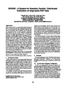
GDQ groups processes together exponentially by weight, such that group G k contains all the processes with weights between 2k (inclusive) and 2k+1 (exclusive) 1 . We call Gk = {C : 2k ≤ φC < 2k+1 } the group of order k, where k is the order of all the processes in G k . The number of groups is denoted by g, and can be at most blog φmax c + 1, where φmax is the maximum possible weight. For example, with 32 bit weights, g ≤ 32. We associate the following variables with a group G: the weight of the group, Φ G , is the sum of the weights of all processes in G; the work of G, WG is the sum of the work of all processes in G. Finally, N k is the number of processes in group Gk . Clearly, ∑Gk N k = N. For the sake of brevity, we will use Xk to mean XGk for any variable X.

weights groups

1234..7 8 ... 15 16 ... G 0G 1 G 2 G 3

G4

31 32

...

63 64

2

31

...

G5

32

2 −1 G 31

Figure 1: GDQ grouping strategy

GDQ also keeps track of the following: Φ T , the total weight, is the sum of all process weights (or group weights); WT , the total work, is the sum of the work of all processes (or groups). When there are at least P 1 henceforth,

except for writing powers of 2, superscript does not denote exponentiation.

4

runnable processes in the system at all times, WT = Pt where t is the elapsed time. According to its weight, any group G k is “entitled” to be serviced by

Φk ΦT

P processors. GDQ attempts to

allocate processors to groups fairly. However, a group’s processor allocation at any time, denoted by P k , must j k m l k k Φk Φk Φk P (floor) and P (ceiling). Unless Φ P ∈ N, P = Pk + 1. GDQ be an integer. Define Pk = Φ P = ΦT T T will then allocate either Pk or P processors to a group depending on the work accumulated by the group so k

far and the state of the scheduler. The P k processors allocated to group Gk are labeled ℘k1 ,℘k2 , . . . ,℘kPk . Groups are organized into a list of size g. Inside groups, processes are organized into queues, which are linked lists. next(C) denotes the process that follows C in the list. A group has P queues, and each queue k

is in general associated with a single processor. ℘(Q) denotes the processor that works on the queue Q, and Q(℘) denotes the queue that processor ℘ works on. Each queue Q keeps track of a current process, denoted by C(Q), which is receiving service from ℘(Q). A per-queue NVT, denoted nv Q , is used as a round counter to advance the NVT of the queue’s processes. All queues of a group are organized into a per-group linked list. The notation introduced is summarized by table 1 in the Appendix.

2.2 Basic Algorithm Instead of binding individual queues to processors and keeping these queues balanced, we keep the groups fixed and distribute the processors among groups. The set of processors allocated to a group will be kept somewhat stable, thus taking advantage of locality and helping service isolation. In general, depending on its weight, a group can have between 0 and P processors allocated. Work balance is achieved by dynamically changing the processor allocation to groups. We first present the GDQ operation under the assumption that the set of processes and their weights remains unchanged. We call steady-state such intervals of time during which the process mix doesn’t change. The GDQ algorithm can be briefly described as a two-level hierarchical scheduler: Inter-group allocation. At any time, each group G k is allocated either Pk or P processors. At certain times, k

a processor is removed from a group that is over-allocated, and moved to a group that is under-allocated, thus balancing work across groups, according to the inter-group scheduler (Section 2.2.1). Intra-group allocation. Let Gk have a processor allocation of Pk . At any time, ∑gi=1 Pk = P if we are assuming a work-conserving system which has at least P processes. The Pk processors that are allocated to group G k will each be responsible for one of the P queues of k

the group. When Pk = P , all the queues are non-empty, and have a processor associated with them. When k

Pk = Pk , all but one of the queues have a processor; one queue will be stalled. This queue may be empty. All other queues are called active. Since all processes within a queue belong to the same group and thus have similar weights, the processor can proceed in a round-robin manner through the queue to select a process to run. To balance the queues of a group, processes may be moved away from the queue that is most behind in

5

terms of its NVT. The intra-group scheduler is described in more detail in Section 2.2.2. 2.2.1

Inter-Group Allocation

Since the inter-group scheduler is oblivious with respect to the intra-group scheduler, we will abstract groups as clients, and assign processing time in accordance with their weight (the group weight). In effect, we are presenting a stand-alone multiprocessor scheduler where clients may run in parallel with themselves (i.e., since clients are really groups here, they may be serviced by several processors simultaneously), which we employ as part of GDQ to manage processor allocation among groups. The algorithm has the following j k l m smoothness property: given a client of weight φ i , it will at any time run on either ΦφTi P or ΦφTi P processors, which is in some sense the best we can do in terms of matching the client’s ideal allocation. The MFQ

scheduler is described below in its most general form, where the entities being scheduled are called ‘clients’. Multiprocessor Fair Queuing (MFQ ). For a client C of weight φC , the virtual finishing time (VFT ) is , where the sum is over periods τ during which φC remains constant. When the defined as FC = ∑τ wC (τ)+1 φC client’s weight is always constant, FC is simply

wC +1 ΦC .

[7] and [11] offer a more detailed discussion of the

notion of a VFT. We now present MFQ below, noting that it clearly preserves the smoothness property: j k For each client i such that φi ≥ ΦPT , we devote ΦφTi P processors to this client and, if ΦφTi P 6∈ N, we create a j k fictitious client of weight φˆ i = φi − ΦφTi P ΦPT which replaces client i in the scheduler. Because of the aforementioned step, we can assume that each client has weight φˆ i
nvMinQ + δ then MinC ← next(C(MinQ))

7

M OVE -P ROCESS(MinC, Q)

8 9

else nvQ ++

10 nvC(Q) ← nvC(Q) + 2k /φC(Q) 11 return C(Q)

The number δ, like the interval length T for the inter-group scheduler, is a parameter of the algorithm. G ET-M IN -Q UEUE (G) finds the queue in the group G who has the smallest NVT. This queue may be either the stalled queue, or may be an active queue. In the latter case, the queue must contain at least 2 processes to be eligible for selection. No such restriction exists for the stalled queue, which is allowed to become empty. M OVE -P ROCESS (MinC, Q) moves process MinC to the queue Q and places it right before the current process, C(Q). MinC becomes the new current process of Q. Since MinQ has at least 2 processes, MinC 6= C(MinQ) and thus it is safe to steal MinC from MinQ. 8

2.3 Feasibility While the weight values assigned to processes in a single-processor environment are essentially unconstrained, this is not the case in a multiprocessor system. Because a process may only receive service from one processor at a time, it is impossible to satisfy a weight assignment that would give a process more than 1/P of all processor resources. Such a weight assignment is said to be infeasible, and is disallowed. Thus, a feasible weight assignment for the processes in the system is one in which φC ≤

ΦT for any process C P

(1)

If a weight assignment is found to be infeasible, it is adjusted to the closest feasible assignment. As a benefit of grouping processes exponentially by weight, we can readily employ the novel weight adjustment algorithm that was introduced in [3]. This algorithm does not need to maintain additional data structures such as sorted lists of weight, and performs fast weight readjustment, with optimal time complexity of only O(P). We have assumed several times in the description of the GDQ algorithm that we have at least one process in each per-processor queue. We now support this assumption by noting that each non-stalled queue will have at least one process provided that N k ≥ P . Since k

k

P


1 k P

for some

Ci ∈ Gk . We refer to process i as being almost infeasible. This does not contradict the feasibility constraint described in Section 2.3, since

φi Φk

≤ P1k will still hold true. However, in the case of almost infeasible processes,

we can use a different approach to bound their error, by noting that before they were running continuously, their error was bounded as in Theorem 3.6, and by running, even though their group-relative error may decrease, their overall error must be non-decreasing. As for processes that are in the same group as almost infeasible processes, their positive error does not grow more than the bound of Theorem 3.6, since, in effect, the almost infeasible processes get their own processors for the duration they are running continuously, and the work of the remaining processors is distributed in the group under the constraints of Theorem 3.6.

3.2 Time Complexity It is crucial that the kernel scheduler have low overhead, regardless of the number of processes that it needs to schedule. It this section we show that Theorem 3.7. GDQ scheduling incurs constant complexity per decision. Proof. Inter-group (MFQ ) allocation At each inter-group subinterval, the processor that is scheduled will need to identify the group of least VFT that is not running. This takes O(g) time , or O(log g) time with more complicated data structures (but in practice, we use O(g)-time solution, since g is here the number of groups, and we need no locking to traverse an array of groups). The number of subintervals is P, so a time interval T is split into more subintervals as P increases. Since we space the subintervals equally, and only one processor schedules at the border of subintervals, there should be no lock contention issues. Note that no matter how large P is, an individual processor will schedule only every T time units. Per processor, this amounts to a O(g/T ) amortized scheduling cost. Intra-group allocation At the intra-group level, the priority queue for NVT is accessed by all processors in a given group, and locking may prove to be too expensive if using a O(log P) complexity heap. Therefore, we use a linked list, with O(P) scheduling complexity. This overhead is incurred by a processor only when 13

it reaches the end of its runqueue. A quick calculation reveals that, in the case when N >> P, the queues are balanced (with less than N/P tasks per queue), and thus the amortized complexity of traversing the list of runqueues is no more than P/(N/P) = P · P/N. Clearly, δ and T provide a trade-off between accuracy and locking overhead. With small δ, intra-group allocation is kept tight, but processes move across queues more frequently. With small T , processor reallocation is more responsive to discrepancies in service allocated to clients of different groups. This keeps the error bounds down (Theorem 3.6), but is expensive: we want to reallocate processors as rarely as possible, since, besides the locking and time complexity overhead of the operation, moving a processor from one group to another migrates many processes among queues within those two respective groups. We expect that this will also hurt cache affinity. Given the form of the error bounds in Theorem 3.6, it seems beneficial to choose δ and T on the same order. However, in practice, δ has a more pronounced effect on the error of a processes, whereas the error introduced by T is spread over many processes in the group. δ should be taken to be a small number. We found that δ = 4 works well in practice. We conclude with a few comments: • The above bounds hold for static process mixes, where no arrivals or departures are expected. This is mostly to keep the analysis clean and compact, and because the measure of fairness used, the service error, is defined assuming that the process is eligible at all times to receive its due allocation. In terms of running time, as mentioned in Section 2.4, we incur a O(P) cost to readjust weights, and a O(g) cost to recompute the processor allocation of groups. Both g and P can be assumed to be constants. • The inter-group MFQ allocator is a generalization of the simple WFQ VFT algorithm ([6]), and is thus a virtual finishing time scheduler. Interestingly, unlike in the uniprocessor case, using virtual start time instead would result in dramatically worse fairness properties (see Note in A.1). We have not attempted to adapt a more complicated, and accurate algorithm such as WF 2 Q, since the number of groups, g, is a constant, and we are more concerned with the synchronization cost of more complex data structures than with the positive error bound.

4 Measurements and Results To demonstrate the effectiveness of GDQ, we have implemented a prototype GDQ CPU scheduler in the Linux operating system and measured its performance. We present some experimental data quantitatively comparing GDQ performance against the standard Linux 2.4 and 2.6 kernel schedulers, and against the O(1) GR3 multiprocessor scheduler ([3]). We have also conducted extensive simulation studies to capture the service error bounds of GDQ. 14

4.1 Simulation Studies We used a simulator for these studies for two reasons. First, our simulator enabled us to isolate the impact of the scheduling algorithm itself from other activities present in an actual kernel implementation. Second, our simulator enabled us to examine the scheduling behavior across hundreds of thousands of different combinations of processes with different weight values. It would have been much more difficult to obtain this volume of data in a repeatable fashion from just measurements of a kernel scheduler implementation. The scheduling simulator measures the service time error, described in Section 3, of a scheduler on a synthetic set of processes. The simulator takes as input the scheduling algorithm, the number P of processors, and a process mix, consisting of a list of process weights. The process mix is provided by a random mix generator, which, given the number of processes N, the total number of weights ΦT , and an upper limit on the process weights (necessary for feasibility purposes), will generate a random list of process weights. The simulator then schedules the processes using the specified algorithm as a real scheduler would, and tracks the resulting service time error. The simulator runs the schedule, then computes the maximum (most positive) and minimum (most negative) service time error for the given set of processes and weight assignments. This process of random weight allocation and scheduler simulation is repeated for the specified number of process-weight combinations. We then compute the worstcase maximum service time error and worst-case minimum service time error for all processes during all specified number of process-weight combinations to obtain a “worst-case” error range. To measure proportional fairness accuracy, we ran simulations for each scheduling algorithm on 24 different combinations of N and ΦT : the number of number of processes ranges exponentially from 512 to 16384 and the total weight ranges exponentially from 32768 to 262144. For each pair (N, Φ T ), we ran 500 process-weight combinations and determined the resulting worst-case errors overall from the 500 runs. We measured the service error for P = 1, 2, 4, 8, 16, 32, 64, 128. We used δ = 4. To understand the effect of the inter-group time quantum T on the service error, we used T = 20, 40, 80, 160, 320, and 640. We found that the error of GDQ does not get worse as the number of processes increases with Φ T kept constant, and, in fact, for most values of P the error actually improves as N grows, mainly because with more processes and a fixed total weight, the weight skew among processes becomes less accentuated. Figure 2 shows that for fixed values of T , the negative error improves slightly as the number of processors increases, while the positive error gets slightly worse, but keeps well below the theoretical bound of Theorem 3.6. On one hand, the error ought to get better as P grows, since more queues are serviced simultaneously. On the other hand, increasing P means that the process weight upper bound decreases according to the feasibility constraint, and hence there will be more processes in the largest order group. This accentuates the weight skew among groups, causing the inter-group error (which depends on T ) to increase. To put results in perspective, we include the error bounds obtained for the same simulations for the uniprocessor schedulers SFQ ([8]) and

15

100

GDQ (T=20) GDQ (T=80) 1000 GDQ (T=320) SFQ WFQ 100

10

10

1

1

Service Error

1000

1

2

4

8

16

32

64

128

Number of Processors

GDQ (T=20) GDQ (T=80) GDQ (T=320) SFQ WFQ

1

2

4

8

16

32

64

128

Number of Processors

Figure 2: Service error for GDQ with T = 40, 160, 640 when P ranges from 1 to 128, and for SFQ and WFQ when P = 1. Both axes are logarithmic. Left: Positive error. Right: Absolute value of negative error.

WFQ ([11]). The overall error bounds for these common uniprocessor schedulers are substantially worse than GDQ for any number of processes.

4.2 Linux Kernel Measurements We also conducted detailed measurements of real kernel scheduler performance by comparing our prototype

GDQ Linux implementation against the the O(1) GR 3 multiprocessor scheduler ([3]), as well as the standard single queue Linux 2.4 scheduler, and the distributed queue Linux 2.6 scheduler. In particular, comparing against the standard Linux scheduler and measuring its performance is important because of its growing popularity as a platform for server as well as desktop systems. The experiments we have done quantify the scheduling overhead of these schedulers in a real operating system environment. We conducted a series of experiments on an 8-processor system to quantify how the scheduling overhead for each scheduler varies as the number of processes increases. Each process executed a simple microbenchmark which performed a few operations in a while loop. A control program was used to fork a specified number of processes, all having the same weight. Once all processes were runnable, we measured the execution time of each scheduling operation that occurred during a fixed time duration of 3 minutes. This was done by inserting a counter and timestamped event identifiers in the Linux scheduling framework. The measurements required two timestamps for each scheduling decision, so measurement errors of 70 cycles are possible due to measurement overhead. We performed these experiments on the standard Linux 2.4 and 2.6 schedulers, and on the the GR3 and the GDQ prototypes, for up to 1000 running processes. The system was provisioned with either 2 or 8 CPUs. GDQ used T = 20. As shown in Figure 3, the scheduling overheads of Linux 2.6 and GDQ are roughly constant as the number

16

of processes grows. Both schedulers use O(1) algorithms to pick the next process. The highly optimized Linux 2.6 scheduler (which, however, is not a proportional share scheduler) is about 10% faster than GDQ. GR 3 , also a O(1) scheduler, is worse than GDQ because it uses a single queue. Even for as few as 8 procesors, where there is little lock contention, the sched-

Scheduling Overhead (Cycles)

3500 3000 2500

uler pays the memory latency cost for grab-

GDQ (P=8) Linux 2.6 (P=8) GR3 (P=8) GDQ (P=2) Linux 2.6 (P=2) GR3 (P=2)

bing global locks. The Linux 2.4 scheduler has overhead linear in the number of processes, orders of magnitude larger than the schedulers plotted in Figure 3.

2000

To get a rough idea as to how the sched1500

ulers scale with the number of processors,

1000

we compare the scheduling overhead of GDQ

500 100 200 300 400 500 600 700 800 900 1000 Number of Clients

Figure 3: Experimental average scheduling overhead in CPU cycles for GDQ, GR3 , and Linux 2.6 on 2 and 8 processors.

Linux 2.6, and GR3 , using 2 and 8 processors. The centralized queue GR3 scheduler incurs much more overhead especially with 8 processors given its increased synchronization costs. Our GDQ prototype incurs slightly more overhead than the optimized Linux 2.6 scheduler, but provides the benefit of proportional shar-

ing. Both schedulers demonstrate good scalability between 2 and 8 processors.

5 Related Work Most commercial operating systems today sport multiprocessor schedulers of varying degrees of complexity. Most of these are built around heuristics that tackle the trade-offs between response time, throughput, and efficiency ([15]). These algorithms do not implement fair-share scheduling even on single processor machines, and rarely do they achieve at least long-term proportional sharing. On multiprocessor systems, Solaris 2.x uses a global dispatch queue from which it schedules processes. Recognizing the potential bottleneck inherent in such approaches, Digital UNIX keeps per-processor queues, and re-balances the queues regularly. The Linux 2.6 kernel is similar ([10]), except Linux uses the SVR4 priority arrays to help each processor schedule in constant time (under the assumption that there is a fixed, narrow range of allowable task weights). An interesting approach to processor allocation, somewhat related to GDQ, is taken by the Mach operating system. Mach allows applications to create processor sets, which contain a certain number or processors and threads. A processor in a set only works on threads within that set, but processors may move from set to set. The Mach motivation for grouping processors is flexibility in resource management and service guarantee, which GDQ 17

achieves indirectly in the context of proportional sharing. Because of the control it offers to resource allocation and its intuitive fairness model, proportional sharing has been widely studied and applied to both processor and network traffic scheduling. To relate GDQ to the very extensive literature on single resource proportional scheduling, we point the reader to [3]. The problem of proportional multiprocessor scheduling has received significantly less attention, mainly due the extra complications introduced by weight infeasibility, task parallelization, and inter-processor coordination. The solutions proposed so far rely on a single global queue for scheduling, and thus scale poorly. [4] presents

SFS, a multiprocessor extension of the SFQ algorithm ([8]), which performs well in practice but has no theoretical fairness bounds. GR3 , introduced in [3], was the first scheduler providing strong fairness bounds with lower scheduling overhead. SFS introduced the notion of feasible tasks along with a O(P)-time weight readjustment algorithm, which requires however that the tasks be sorted by their original weight. By using its grouping strategy, GR3 performs the same weight readjustment in O(P) time without the need to order processes, thus avoiding the O(log N) overhead per maintenance operation. Since GDQ uses the same task grouping strategy as GR3 , it benefits from the same efficient weight readjustment algorithm. In the context of link scheduling, [2] considers aggregated links, the analogue of multiprocessors for the network server problem, and presents a global queue algorithm that approximates the idealized fluid GPS model for multi-server systems. Their adaptation of WFQ ([11]), called MSFQ, and of WF 2 Q ([1]), called

MSF2 Q, preserve the error bounds of WFQ (-1 to N) and of WF 2 Q (-1 to +1) respectively whenever the flows are backlogged at all times. Otherwise, with an unlucky interplay of busy periods, the service error can be as small as −P, as big as +P for MSF2 Q. MSFQ ’s positive error bound is presumably N + P is such a case. We note that the O(P) error is unavoidable in any system where flows are not backlogged at all times (correspondingly, tasks are not runnable at all times). Since the model of aggregated network links allows for packets of the same flow to be serviced at the same time, the single resource algorithms cannot be adapted in the same way to multiprocessor scheduling. Even for the case of the GDQ inter-group scheduler, where tasks of the same group may run in parallel, we could not use the algorithm of [2], as that would not guarantee a ΦG G share of b Φ ΦT Pc or d ΦT Pe to group G at all times (the smoothness property).

Multi-resource scheduling has been receiving some attention outside of the proportional sharing paradigm as well. In the periodic task model, [13] looks at providing fairness on multiprocessor systems and, while noting the benefits of distributed queues, contends that a global queue is simpler to design and implement. The authors review some approaches to periodic task scheduling on multiprocessor systems, in particular flavors of the p-fair scheduler, and extend the work on p-fair multiprocessor scheduling in [12]. [5] shows how to adapt a p-fair scheduler in a work-conserving operating system scheduler. [16] targets programmable network routers, and tries to efficiently use the very small instruction cache by keeping packets that use same code on the same processor, and processing them back-to-back. They note the conflicting requirement in scheduling packets to optimize delay or cache affinity. [14] considers cache affinity in relation to multiprocessor scheduling. Cache 18

performance is an important factor of system performance, and a distributed queue approach has the implicit benefit of reusing much more cache state than a global queue design. Given that resources may be poorly used if allocated independently, [17] attempts to combine processor and link scheduling in programmable multiprocessor network routers. An operating system presents similar challenges. While GDQ considers cache performance as one of its design motivations, explicitly taking into account memory, disk, or network activity is beyond the scope of this process scheduling algorithm.

6 Conclusions and Future Work We have designed, implemented, and evaluated Grouped Distributed Queues scheduling in the Linux operating system. We prove that GDQ is the first and only O(1) distributed queue multiprocessor scheduling algorithm that guarantees a constant service error bound compared to an idealized processor sharing model, irrespective of the number of runnable processes. Previous approaches to multiprocessor scheduling used single, centralized queues, or relied on heuristics that did not even provide long-term fairness. To achieve good proportional share fairness with low overhead, GDQ employs an exponential grouping strategy and uses a two-level hierarchical scheduler. GDQ introduces a new way to consider the pairing of processors and queues and presents a virtual-time-based inter-group scheduling algorithm with good fairness and smoothness properties. For each processor, GDQ uses a fair and efficient intra-queue round robin scheme. We have measured the performance of GDQ using both simulations and kernel measurements of a prototype Linux implementation. Our simulation results show that GDQ can provide good proportional fairness behavior even as the number of processes exceeds 250,000. Our experimental results using our GDQ Linux implementation further demonstrate that GDQ provides accurate proportional fairness behavior on real applications with comparable scheduling overhead to the O(1) Linux scheduler. While GDQ is a distributed queue scheduler, there is a fair amount of communication and process exchange among processors and their queues. Re-balancing less often and using less information would have beneficial effects on the synchronization overhead. A major advantage of distributed queue scheduling lies in benefiting from cache state by keeping processes on the same processor for a long time. Making caching explicit in the scheduler would be worthwhile.

References [1] Jon C. R. Bennett and Hui Zhang. WF2 Q: Worst-Case Fair Weighted Fair Queueing. In Proceedings of IEEE INFOCOM ’96, pages 120–128, San Francisco, CA, Mar. 1996. [2] Josep M. Blanquer and Banu Ozden. Fair Queuing for Aggregated Multiple Links. In Proceedings of ACM SIGCOMM ’01, pages 189–198, San Diego, CA, Aug. 2001.

19

[3] Bogdan Caprita, Wong Chun Chan, Jason Nieh, Clifford Stein, and Haoqiang Zheng. Group Ratio Round-Robin: O(1) Proportional Share Scheduling for Uniprocessor and Multiprocessor Systems. In Proceedings of the 2005 USENIX Annual Technical Conference, pages 337–352, Anaheim, CA, April 2005. USENIX. [4] Abhishek Chandra, Micah Adler, Pawan Goyal, and Prashant J. Shenoy. Surplus Fair Scheduling: A ProportionalShare CPU Scheduling Algorithm for Symmetric Multiprocessors. In Proceedings of the 4th Symposium on Operating System Design & Implementation, pages 45–58, San Diego, CA, Oct. 2000. [5] Abhishek Chandra, Micah Adler, and Prashant Shenoy. Deadline fair scheduling: Bridging the theory and practice of proportionate fair scheduling in multiprocessor systems. In RTAS ’01: Proceedings of the Seventh Real-Time Technology and Applications Symposium (RTAS ’01), page 3, Washington, DC, USA, 2001. IEEE Computer Society. [6] A. Demers, S. Keshav, and S. Shenker. Analysis and Simulation of a Fair Queueing Algorithm. In Proceedings of ACM SIGCOMM ’89, pages 1–12, Austin, TX, Sept. 1989. [7] S. J. Golestani. A Self-Clocked Fair Queueing Scheme for Broadband Applications. In Proceedings of IEEE INFOCOM ’94, pages 636–646, april 1994. [8] P. Goyal, H. Vin, and H. Cheng. Start-Time Fair Queueing: A Scheduling Algorithm for Integrated Services Packet Switching Networks. IEEE/ACM Transactions on Networking, pages 690–704, Oct. 1997. [9] L. Kleinrock. Computer Applications, volume II of Queueing Systems. John Wiley & Sons, New York, NY, 1976. [10] Robert Love. Linux Kernel Development. SAMS, Developmer Library Series, first edition, 2004. [11] A. Parekh and R. Gallager. A Generalized Processor Sharing Approach to Flow Control in Integrated Services Networks: The Single-Node Case. IEEE/ACM Transactions on Networking, 1(3):344–357, June 1993. [12] A. Srinivasan and J. Anderson. Fair scheduling of dynamic task systems on multiprocessors, 2003. [13] A. Srinivasan, P. Holman, J. Anderson, S. Baruah, and J. Kaur. Network Processor Design: Issues and Practices Volume II, chapter Multiprocessor Scheduling in Processor-based Router Platforms: Issues and Ideas. Morgan Kaufamann Publishers, 2004. [14] Josep Torrellas, Andrew Tucker, and Anoop Gupta. Evaluating the performance of cache-affinity scheduling in shared-memory multiprocessors. J. Parallel Distrib. Comput., 24(2):139–151, 1995. [15] Uresh Vahalia. UNIX Internals: The New Frontiers. Prentice Hall, Upper Saddle River, NJ, 1996. [16] T. Wolf and M. Franklin. Locality-aware predictive scheduling for network processors. In Proc. of IEEE International Symposium on Performance Analysis of Systems and Software (ISPASS), pages 152–159, Tucson, AZ, Nov. 2001. [17] Yunkai Zhou and Harish Sethu. On Achieving Fairness in the Joint Allocation of Processing and Bandwidth Resources: Principles and Algorithms. Technical Report DU-CS-03-02, Drexel University, Jul. 2003.

20

A

Appendix

A.1 Terminology Term

Description

Term

Description

Process j.

φC

The weight assigned to process C.

φi

Shorthand notation for φCi .

σC

The order of process C: blog φC c.

N

The number of runnable processes.

Cj

2k

φ max

Group of order k, {C :

ΦG

The group weight of G: ∑C∈G φC .

Φk

Nk

P

Pk

Number of processes in group Gk . k j Φk P . ΦT

P

Pk

Number of processors assigned to group G k .

℘j

jth processor.

℘kj

jth processor of group Gk .

wC

The work of process C.

WG

The group work of group G. The VFT of group G.

≤ φC
nvQ3 + δ. Therefore, ℘2 steals process C6 from Q3 and runs it, incrementing its NVT to 1. At time t + 4, ℘3 is at the end of its round, increments nv Q3 to 2, and runs C8 , whose NVT becomes 6/3. ℘1 is also at the end of a round, increments nv Q1 to 3, runs C4 and increments its NVT to 3. ℘2 still runs process C6 , incrementing its NVT to 2, since its NVT is smaller than the queue NVT, which is 3. p1 1 4 1

p1 1 4 1

5 0

p2 1 7 1

p1 2 4 2

5 1

p2 2 7 2

p3 1 8 2/3 9 0

6 0

p3 1 8 4/3 9 0

t

6 0

t+1

p1 2 4 2

5 2

p2 3 7 3

p2 3 7 3

6 1

p3 1 8 4/3 9 2/3 6 0

p3 1 8 4/3 9 4/3

5 1

t+2

t+3

p1 3 4 3

5 2

p1 3 4 3

5 3

p1 4 4 4

5 3

p1 4 4 4

5 4

p2 3 7 3

6 2

p2 3 7 3

6 3

p2 4 7 4

6 3

p2 4 7 4

6 4

p3 2 8 6/3 9 4/3

S 2 8 6/3 9 4/3

t+4

t+5

p1 4 4 4

5 4

8 8/3

p1 4 4 4

p2 4 7 4

6 4

9 6/3

p2 4 7

t+8

p1 5 4 5 p2 5 7 5

5 5 6 4

S 2 8 6/3 9 4/3 t+6

5 4

4 6 4

p1 5 4 5

9 12/3

p2 5 7 5

t+7

8 10/3

p1 4 4 4

5 4

8 12/3

p1 5 4 5

5 4

8 12/3

9 8/3

p2 4 7 4

6 4

9 10/3

p2 4 7 4

6 4

9 12/3

t+9 8 12/3

S 2 8 6/3 9 4/3

t+10 5 5 6 5

8 14/3

p1 5 4 5

9 12/3

p2 5 7 5

5 5 6 5

t+11 8 16/3

p1 6 4 6

8 16/3

9 14/3

p2 5 7 5

6 5

9 16/3

p4 6 5 6 t+12

p1 6 4 6

8 18/3

p2 6 7 6

6 5

p4 7 5 7 t+16

t+13

9 16/3

p1 7 4 7

8 18/3

p2 6 7 6

6 6

p4 8 5 8

t+14

9 16/3

t+15

p1 7 4 7

8 20/3

p1 7 4 7

8 22/3

p2 6 6 6

9 18/3

p2 7 6 7

9 18/3

7 7

p4 8 5 8

7 8

p4 8 5 8

t+18

t+17

t+19

Figure 5: Intra-group scheduling example. The group considered is G 2 , having processes C4 , C5 , C6 , and C7 of weight 4, and C8 and C9 of weight 6. For each time unit, the three queues Q 1 , Q2 , and Q3 are displayed (unless Q3 is empty). For each queue, we list the processor working on that queue (‘S’ means stalled), the current NVT of the queue, followed by the list of processes. Each process is represented as a box containing the process number (in bold face) and the process NVT. At time t + 5, processor ℘3 is reassigned to G1 , so Q3 becomes stalled. From time t + 5 to t + 7, ℘1 and ℘2 round-robin between C5 , C4 , and C6 , C7 respectively. 24

At time t + 8, both queues will be at the end of the round, with their queue NVT s being 4. This is more than nvQ3 + δ = 2 + 1, hence Q1 steals C8 and Q2 next steals C9 from the stalled queue, which becomes empty. Up to time t + 14, ℘1 round-robins between C4 ,C5 ,C8 and ℘2 round-robins between C6 ,C7 ,C9 . At time t + 15, ℘4 gets assigned to G2 , and will grab the next process of Q1 , which is C5 , and run it. Later, at time t + 18, Q3 ’s NVT will be 8 at the end of a round, while Q 2 ’s NVT will be 6. ℘4 will therefore grab the next process of Q 2 , C7 in this case. After this, the composition of the queues will be Q1 = {C4 ,C8 }; Q2 = {C6 ,C9 }, Q3 = {C5 ,C7 }. We notice that the queues have managed to arrive at an optimal weight balance for the given mix as the algorithm ran. Figure 5 illustrates this example.

A.3 Proofs In the appendix we include all of the omitted proofs. We repeat the claims also.

Lemma 3.1. Consider any scheduling point t, and let the client selected be j. If at point t, some client i is such that

wi (t)+δi φi