tions for assayists and laboratory managers on good practice in data processing ... analysis that is desirable in programs, with some approxi- mate mathematical.
CLIN. CHEM. 31/8,1264-1271 (1985)
Guidelines for Immunoassay Data Processing1 R. A. Dudley,2 P. Edwards,3
R. P. Eklns,3 D. J. Flnney,4 I. G. M. McKenzie,4 G. M. Raab,4 D. Rodbard,5 and
R. P. C. Rodgers6 These guidelines outline the minimum requirements for a data-processing package to be used in the immunoassay laboratory. They include recommendations on hardware, software, and program design. We outline the statistical analyses that should be performed to obtain the analyte concentrations of unknown specimens and to ensure adequate monitoring of within- and between-assay errors of measurement.
AddItIonal Keyphrasee: statistics programs data processing
Third, machine computation .
quality control
computer
The authors of this paper were convened as a group by the International Atomic Energy Agency to make recommendations for assayists and laboratory managers on good practice in data processing for radioimmunoassay and related techniques. They were requested to identify those computational procedures that are appropriate, especially in a hospital laboratory providing a routine service, and to establish priorities as to their importance. It is timely to examine this topic. In recent years the dramatic increase in power and decrease in price of computing hardware have brought the capability of machine computation within the reach of all laboratories, either as an integral part of a sample counter or as an independent device. Many programs have been designed, thus testing a diversity of approaches but subjecting the user to a bewildering choice among possibilities. In the opinion of this group, most commercially available programs for analyzing immunoassays lack essential features. Indeed, several prograins that have been developed for programmable calculators (1,2) show more sophistication than those supplied as “black box” systems by many manufacturers of beta- and gamma-counters. The group agreed on several general principles. First, all aasayists can benefit from the computational and statistical 1 This article should be regarded as the composite view of a committee of experts, convened by Dr. B. A. Dudley under the auspices of the International Atomic Energy Agency, Vienna, Austria. It is neither an “official” position of the IAEA nor a formal policy of the AACC. However, it should serve to stimulate thinking by all in the RIA and immunoassay fields. We hope it will contribute to an improvement in the overall quality of software systems for these kinds of analyses. 2 International Atomic Energy Agency, Wagramerstrasse 5, P.O. Box 100, A-1400 Vienna, Austria. 3Department of Molecular Endocrinology, Middlesex Hospital, London, U.K. 4 of Edinburgh, Edinburgh, U.K. Institute of Child Health and Human Development, National Institutes of Health, Building 10, Room 8C413, Bethesda,
MD 20205.
6University of California, San Francisco, CA. Received February 5, 1985; accepted May 31, 1985. 1264
procedures that a good program can offer.Indeed, the less statistically experienced the user, the more he stands to gain by such assistance. Second, while one goal of computation obviously is to derive the concentration of analyte in the samples measured, the main advantages of machine computation include automation, speed, improved accuracy (through avoidance of gross errors), and detailed statistical analysis and accounting of sources and magnitude of errors.
CLINICALCHEMISTRY,Vol.31, No.8, 1985
should never be thought
to
relieve the analyst of responsibility for the reliability of his measurements; all it can do is provide results that are computationally sound, that are relevant to the assessment of reliability, and that are displayed in the most comprehensible manner. Fourth, the creation of suitable programs is a major task that can be accomplished successfully only through the combined efforts of professional analysts, statisticians, and programmers. Finally, although the user himself need seldom know the details of the mathematical analysis, it is improper that proprietary secrecy should conceal the basic strategy, algorithms, equations, and assumptions. Two restrictions adopted by the group as to the scope of this paper should be stressed. First, it is not a general critique of quality control. Although data processing is one key element in quality control, the latter field embraces much more than data processing. Second, being directed at the practicing assayust and laboratory manager, the paper does not offer detailed algorithms such as would be required by a programmer. Instead, we seek to explain the type of analysis that is desirable in programs, with some approximate mathematical amplification in appendices to sharpen the concepts.
Hardware and Software The choice of a computer system for a particular laboratory will depend on several factors. The most important factor is that the system be able to run a data-analysis package that at least meets the minimum requirements set out here. Secondly, in terms of capacity and speed it must be able to handle the volume of work done in the laboratory. In all cases the system should be tailored to fit the needs of the laboratory and be regarded as a piece of equipment that is as essential as a gamma counter or a centrifuge. Our minimum recommendation would be a computer with 48K of memory and one or more disk drives. For two reasons we do not consider programmable calculators in any detail here. First, the best of the existing programs are near the limit of their capacity (1,2) and, second, the calculators can now be replaced by very-low-cost microcomputers. The development of adequate software is a difficult and time-consuming task and should not be undertaken lightly. If possible, good existing software should be adopted. Unless
the user is willing to accept a program that will be usable only during the lifetime of a particular machine, the following criteria should be met: Programming language: The program should be written in a standard version of a well-established programming language (e.g., FORTRAN, BASIC, or PASCAL) and in general should avoid machine-specific “enhancements.” However, some machine-specific features will often be necessary and some “enhancements” may be desirable. Modularity: The program should consist of well-defined modules, each performing a few specific tasks. This allows existing modules to be replaced by new modules if better algorithms become available, and modules containing new features can easily be added. All machine-specific features and “enhancements” should be placed in well-defined and documented modules so that they can be readily adapted to new hardware or new operating systems. Operating systems: The problem of moving from one machine to another may be minimized by a good choice of operating system. Some operating systems can be used on machines of different power, and a judicious choice allows a laboratory to upgrade its computer requirements with minimum dislocation. Examples of such systems are CP/M, MS/ DOS, the ucun p-system, unix, and PICK. Documentation: Program documentation should always be clear and detailed. Internal documentation should be adequate to facilitate program modification. All algorithms should be publicly available so that they may be examined and, where necessary, criticized. A manufacturer unwilling to do this should provide a full description of the methods used, including appropriate references to the literature and specimen analyses of several real data sets that illustrate all the features of the program. Good documentation on the use of the programs and on the interpretation of the output is essential. Graphics: The use of high-resolution graphics is perhaps the only place where the use of machine-specific “enhancements” to standard programming languages is justifiable, because good graphical output is frequently clearer than any other representation of information. However, such output should always be included in separate modules, and alternative replacement modules, with low-resolution graphics produced by a standard printer, should be available. In the absence of an adequate graphical output, the alternative of alphanumeric output should be made available.
Input and Output Input of Responses The word “response” is used in this report for the quantitative measurement obtained for each sample of standard or test preparation. For techniques that involve radionuclides, the response is “counts”; for other techniques, it might be the reading from a spectrophotometer or some other instrument. Input of responses by direct link from the counter or other device or by machine-readable media, such as paper tape or data-logger cassette, should be the norm for routine assays. Such an approach eliminates operator error during data entry. Even so, some errors can occur, and the program should check that the data have the expected format and magnitude. Occasionally, manual data entry is unavoidable; a thorough check that the entry is correct is then essential. If the computer is connected directly to the measuring device, the responses should be accumulated in a ifie and analyzed as a batch once the assay is complete. This makes data correction easier and allows more satisfactory error analysis and quality-control procedures. Moreover, comput-
ing resources will usually be used more efficiently if data collection can proceed while the computer is being used for other purposes. A printed copy of the stored data ifies must always be available for inspection.
Input of Assay Configuration
and Instructions
For the responses to be analyzed, the program will need information on the concentration of the calibration standards, dilutions of the unknowns, and the order in which the responses are being entered (assay configuration). In addition, instructions are required on the type of analysis required. The program should allow some flexibility in the assay configuration, which includes the identification of quality-control pool samples (see the section on “betweenbatch quality control”). The provision of standardi.zed configurations for certain types of assay is useful, so that only the number of test samples need be entered (3).
Output The details of output from specific parts of the program are dealt with in the appropriate section below. Care should be taken to avoid unnecessary output, which reduces the impact of important information. Numbers should be written in a readable form without the use of exponential format, and the use of numeric codes or cryptic mnemonics should be avoided. Instead, clear, concise messages in ordinary language should be used. If the result obtained from a statistical test on the data from an assay is satisfactory, a simple message may be all that is required. However, more information should be available if a test fails or if the operator requests the information. It may be useful to store such detailed information in a disk file for later inspection if necessary.
Analysis of Responses from a SIngle Assay Batch General Computer programs for the analysis of assay responses fall into two classes. Programs of the first type take a manual (usually graphical) analysis as their starting point. The routines are designed to mimic the procedure that a technician might use with a ruler or a flexicurve. Examples are linear interpolation, smoothing techniques, and some uses of spline functions. Programs of the second type base the analysis on a statistical model of the assay, and thus lead to an assessment of errors of measurement. We are unanimous in recommending a program that uses a statistical model. The basic statistical model of an assay assumes that the response from a particular tube has two components: #{149} The expected response for the tube, which depends only on the amount of analyte in the tube. This is the average response that would be obtained if a very large number of measurements were made for a given dose of the analyte. The relation between expected response and dose is called the dose-response curve or calibration curve. #{149} A random component due to variability in experimental procedures and measurements, which will have an average value of zero across a large set of measurements. It will not be satisfactory to assume that this component has a constant standard deviation at all levels of the response. In most cases, the size of this random component will increase with the level of response. A formulation of how the standard deviation (or some other measure of variability) deponds on the mean response is known as the “response-error CLINICAL CHEMISTRY, Vol.31,No. 8, 1985 1265
relation,” or RER.7 Details of how the RER affects immuneassay results have been published (4, 5, 8). This is an idealized model of an assay, in which the response in one assay tube is unaffected by the responses in neighboring tubes; there are no mishaps that have produced completely erroneous results for certain tubes; no systematic effects are present, such as drift due to time or carrier position; and the expected response is determined only by the concentration of the analyte being measured. However, in practice, satisfactory assays can come close to this ideal. Any serious departure from this idealized model of the assay system may lead to results that are incorrect and subject to much greater uncertainty than the calculations imply. Thus an essential part of the analysis of an assay batch is to check that the responses are consistent with these assumptions about the assay. The extent to which this will be possible will depend on the assay design, which is beyond the scope of this paper but has been discussed elsewhere (6, 7). The steps described in the section on “steps in the analysis below suggest how the analysis of an assay batch can proceed, incorporating checks on the assumptions. We have presented them in one possible sequence, but alternative orderings are possible. ...“
1/ A family of curves in which individual members are defined by the numerical values of very few (preferably only four) parameters. 2/ Flexibility of shape, slope, and position to suit the requirements of standard assay techniques. 3/ Monotonic form (i.e., no reversals of slope), and restraint from making detours for outliers. The “four-parameter logistic” curve appears to be the most generally useful and versatile model that will satisfy the above requirements, although nothing said here implies that it is “right” and all others “wrong.” Its parameters characterize: (a) expected
count at zero dose, not necessarily identical with any one observed count (Figure 1); (b) “slope” factor, related to rate of change of count with increasing dose; (c) the dose expected to give a count halfway between a and d, i.e., the EC or IC; (d) expected count at “infinite” dose (high-dose plateau or asymptote), not necessarily identical with a count for nonspecific binding. The general form of equation then is: Expected
response
at dose
=
d +
+(dose/c)’
Recommended Models Dose-response curve. Numerous models have been sugA standard program should embody one acceptable general-purpose model; a more sophisticated program might include alternatives occasionally needed for special circumstances. Important features of a model suited to wide use in routine assays are: gested.
Abbreviations
used in this paper:
B0, counts observed for zero dose; B/B0, normalized
response
variable, ranging from 0 to 1, representing counts bound above nonspecific, relative to counts bound above nonspecific for zero dose of analyte. Also commonly expressed as a percentage, %B/B0, on a scale from 0 to 100%. B/F, bound-to-free ratio for labeled ligand. BIT, bound-to-total ratio for labeled ligand. %CV, coefficient of variation, as a percentage of the mean. a, b, c, d: parameters of the four-parameter logistic model, with a = expected response at zero dose of analyte; b = slope factor or exponent, with absolute magnitude equal to the logit-log slope; c = EC or IC, i.e., concentration of analyte with an expected response exactly halfway between a and d; d = expected response for infinite analyte concentration (often, though not always, synonymous with nonspecific counts bound). nASA, enzyme-linked immunosorbent assay. EMrr’, enzyme-multiplied immunological technique. IRMA. immunoradiometric assay (generic name for assays involv-
ing labeled-antibody reagents). J, exponent utilized in power function model for response-error relationship. NSB, nonspecific binding. r, number of replicates. RER, response-error relationship, commonly expressed as vanance of the response as a function of expected level of response, e.g. =
ao y’.
RMS, root mean square error. For unweighted regression, the standard deviation of a point around the fitted curve. For weighted regression, the ratio of observed error to predicted error, based on the particular weighting model utilized. sd,standard se, standard
deviation.
We recommend that the RER be expressed as a product of two terms. The first term will be a constant-i.e., independent of the level of response-for a particular assay batch (or for a subset of the batch if standards and unknowns are to be treated separately). The second term will describe how the standard deviation of the responses varies with the level of LOG,0 -I
COUNTS BOUND B
CLINICALCHEMISTRY, Vol.31, No.8, 1985
COUNTS 2
0
3 FR!(
8/T
Bo 2.000
B/U. I #{176}
4
10,000
IO000
I
8
-‘-.,.1eN..
6
PEDjo
-I 6
‘#{176}“0
2,000
e000
4.000
6,000
2
4
4.000
1
.2
N 2.000
0
0
0
error.
y’, slope. residual mean square between doses. 5, mean square within doses. w, weight for observation i. z, estimate of log(dose). 1266
This curve (Figure 1) satisfies all the desiderata and is adequate for the vast majority of existing immunoassay systems. It is continuous and smooth, and the slope factor is very stable in repeated assay batches. It can approximate closely the simple mass-action equation (8). One additional parameter for “asymmetry” is easily incorporated to give even greater versatility (9, 10). Response curves are further discussed in Appendix 1, and greater detail can be found elsewhere (11, 12). Response-error relation (RER): Detailed modeling of experimental errors and their sources is not required. A program should include a simple formulation of how the variance or the standard deviation of the random component of the response varies with the mean response level. This will usually require no more than two parameters (e.g., a power function, a linear or quadratic relationship for the standard deviation or the variance as a function of expected response).
le
: .‘#{176}!!
0IO
!‘!“‘“!
1
d.O.(flO.Oec,GccJ
.iei I
Fig. 1. Schematic
16,000 18.000
-
20,000
1,
I 10
DOSE
-
-19-
00
1000
22,000.1
S (104 scsI.)
drawing of a dose-response (calibration) curve
Note smooth, symmetrical sigmoidal shape, characterized by four parameters (a. b, C, c. Confidence limitstaper in a smooth, consistent manner. Reproduced, with permission, from ref. 29
the response,
and this relationship will remain fairly conacross a series of batches (assays). This implies that the scale of the random errors in the responses may differ between batches, but that the shape of their relationship to the mean response would be similar in each batch (4, 5). An appropriate shape for the dependence of the standard deviation on the mean response should be determined from the data for a series of assays. This information is fed back into the program either: #{149} by the user entering a few numbers (preferably just one) calculated from a series of assays, or #{149} preferably, by the computer performing this automatically by utilizing stored information from previous batches. Poisson errors due to counting may be estimated directly from the number of counts and the RER can, if desired, be specified without this component. The counting error can then be added to the estimated RER to obtain the total error (13). Details of how to characterize the RER are given in Appendix 2. stant
Steps in the Analysis of a Single Batch Adjustment and verification of responses. Certain procedures may yield responses that require adjustment before calculation starts. For example, variable counting efficiency as a result of variable quenching in liquid-scintillation counting gives a response that must be corrected before other calculations. Other adjustments, however, such as variable recovery in preliminary separation procedures, must be made after the concentrations have been estimated. The computer program should be designed to handle any such procedure that the laboratory methods demand. It may be useful to display any apparent anomalies in the data-such as serious discrepancies among replicates from the same sample or inconsistent standard responses-before the main analysis is undertaken. Error correction can be done at this stage, but a record of any changes should be sent to the quality-control file (see below) and must be recorded on the output. Screening of replicate sets. When some or all of the specimens have been measured in replicate, the RER may be estimated from the scatter of the sets of replicates, which may thus enable individual “outliers” to be detected. The term “outlier” is used with two different meanings in immunoassays. Firstly, the term “outlier” has been used to denote a member of a set of replicates that is dramatically further from the set mean than would be expected from the estimated HER, and presumably indicates a blunder. We use it in this sense here. Secondly, the term is used for the case when all the responses for a concentration of standard deviate from their expected value. This case is dealt with in the section on “testing goodness-of-fit.” The first step is to use the data from the replicate sets to estimate the HER. Where the shape of the HER can be assumed to be constant over a series of assays, only the multiplying constant needs to be found. This is easily estimated as a weighted combination of the individual variances. Practical difficulties can arise if any gross outliers are present in the data. Robust techniques, such as taking medians within sub-groups (5) or a modification of the method proposed by Healy and Kimber (14), should prevent these extreme sets from influencing the estimates. After the RER is estimated from all the data, the scatter of individual sets of replicates about their mean can be compared with what would be expected from the RER. All sets where the ratio of observed to expected variance is greater than some value that would be very unlikely to occur by chance (say, p 3.0 warns of poor fit at that dose. A plot of the standard responses and the fitted curve resembling Figure 2 will be a useful diagnostic tool for the assayist. It will help to reveal whether there is a systematic lack of fit-perhaps caused by an unsuitable choice of model for the dose-response curve-or whether responses at one or two dose levels are grossly out of line. The latter situation corresponds to the second usage of the term “outlier,” meaning inconsistent results from one standard dose relative to other doses, rather than a response inconsistent with other replicates at a single dose. Automatic rejection of all the responses from one standard dose is not recommended, there seldom being enough doses to make such a procedure reliable. A minimum of eight dose levels is recommended. Manual intervention should be allowed to reject an occasional standard dose (but never more than one) on the basis of a mixture of statistical grounds and laboratory experience. Excessive manual rejection, however, will lead to biased, over-optimistic estimates CLINICAL CHEMISTRY, Vol.31,No. 8, 1985
1267
-1
3
Logl(X)
Fig. 2. Computer generated plot ofthestandardcurvedata,thefitted logistic curve,andthe 95% confidence limits for a single observation, (excluding uncertainty inthe position ofthecurve) From IBM-PC RIA program ofM. L Jaffe
of precision. Finally, the program
should produce a table showing the of analyte in the standards when these are treated as if they were unknown specimens. Comparison of these results with the actual concentrations of the standards will suggest how much bias a misfitting dose-response curve might introduce into the estimates for the unknowns. A statistically significant lack of fit, especially in assays of high precision, may be sufficiently small that the results will remain useful for their intended purpose. Presentation of precision profile. The above estimation of the HER provides the program with an estimate of the random error at any level of response. The combination of this estimate with the slope of the fitted dose-response curve permits one to obtain an estimate of the random error in the estimated concentration of an unknown (Appendix 3). A representation of this derived variability in the estimated concentration of unknowns against analyte concentration is known as the precision profile. (The term “imprecision proffle” is also used, to emphasize that a larger percentage coefficient of variation indicates poorer precision.) This should be presented either as a graph (Figure 3) or as a table of expected precision (e.g., the percentage coefficient of variation or standard error for a test preparation) vs concenapparent
concentration
tration.
0.1
1
10 hCG (ngimi)
100
1000
Fig. 3.“Precision profile”: %CVforan unknown specimenmeasured in duplicate (ordinate) plotted vs serum analyteconcentration (logscale) on the abscissa (3( The effects of uncertainty in the positionof the standardcurveare not included in this example. Also shown: empirical within-batch %CV(#{149}) andbetween-batch %CV (o)for three quality-controlpools, analyzed in triplicate in each of the past 20 batchesor assays 1268
CLINICAL CHEMISTRY, Vol.31,No. 8,1985
Precision profiles can be calculated for a single measurement for the unknown, or for the mean of duplicate or triplicate measurements. The error in estimating the response curve may or may not be included in the errors used to calculate the precision profile: this option should be specified. The program should generate a table or graph of the precision proffle for the number of replicate measurements and the sample volume ordinarily used for the unknowns. The program should also provide an estimate of the lowest level of reliable assay measurement. A statistical estimate of the minimal detectable concentration (18) is recommended. Alternatives recently described by Oppenheimer et al. (19) may be useful. Estimation of concentration for test samples (unknowns). The program must provide an estimate of the concentration of each unknown sample and a measure of its precision. The precision may be expressed as an estimated percentage error in the result (% CV) from the precision profile, or as 95% confidence limits. A warning when the estimated error exceeds a certain threshold (e.g., 10%) is useful, and may be all that is required for certain applications. When a sample is analyzed in replicate at a single dilution, the concentration corresponding to the mean response is read from the calibration curve and corrected for sample dilution. The estimated precision at this level of response is used to assign confidence limits or a %CV to the result. lithe sample has been included at two or more dilutions, a combined estimate of concentration should be obtained from all the responses by using a weighted average, which gives greater influence to the doses that lie within the region of the curve where estimation is more precise. Again, estimates of precision should be obtained for this combined estimate. When two or more dilutions are included, the program can test whether the concentrations obtained at different parts of the response curve are consistent. This is a generalized test of “parallelism.” An outline of these calculations is given in Appendix 4. For each test sample, the minimum output from the program should be an estimated concentration, along with warning messages about outliers, lack of parallelism, or poor precision. For outliers or lack of parallelism, the estimates from individual responses or individual doses will help the assayist to interpret the results. Evaluating assay drift or instability. Appreciable drift in responses from the same sample placed in different positions in the assay batch may seriously invalidate the estimates of precision described above. Information will be available from replicate counts from standards or unknowns placed in different parts of the sequence of test samples. Tests of possible distortion of results caused by systematic drift can be based upon these replicate responses (or upon the corresponding estimates of concentrations). The particular test adopted will depend on the assay design, but will usually consist of a regression analysis or an analysis of variance with suitable weighting. A combined test should make use of all the available data. Any apparent drift should be evaluated in terms of its effect on the estimated concentrations, so that its importance may be assessed.
Between-Batch Quality Control One important goal of data analysis is to reveal whether performance is consistent in a series of assay batches. Automated data analysis is essential if a sufficiently broad set of indicators is to be followed without excessive labor. An archive should be maintained for the most important indices of consistency, including the results from qualitycontrol pools, the parameters of the dose-response curve, the
RER, the weighted root mean square error, and a summary of rejected data. Although subsequent analysis of results from qualitycontrol pools may be carried out by a separate program, this should not be optional. Recommendations on the placing of the quality-control pools in the assay batch and their disposition at different analyte concentrations have been made elsewhere (20), although guidelines are somewhat arbitrary. Use of at least three quality-control pools, with different analyte concentrations, is recommended. The results from these pools should be analyzed for trends or sudden shifts between batches. The analysis should include the use of control chart methods, mean squared successive differences, or other appropriate tests for randomness. Details of these methods are discussed in standard texts (21, 22) and their application to immunoassays has been discussed (23-25). Similar tests can also be applied to other features of the assay such as the parameters of the standard curve, but these will be of secondary importance. The program should provide tests that combine information from all the quality-control pools. These test whether all the pools are changing in a similar manner. In their simplest form they can be performed by applying the tests above to the mean of all the quality-control pools; weighting according to the estimated precision of each pool is desirable. Assessment of between-batch precision. The quality-control specimens are the only source of information on between-batch precision, which is the essential measure that a clinician needs for comparing results obtained on different days. The between-batch precision includes components from within-batch errors and between-batch errors. The program should compute the estimated betweenbatch precision for each quality-control pool. Two components of between-batch imprecision can be predicted from the responses from a single batch. The first is the withinbatch variability for each specimen. A second is due to the uncertainty in the position of the fitted dose-response curve as a result of the variability in responses for the standards. Both of these components can be estimated from the data from a single batch, although the second component, which is relatively small, is part of the between-batch variation as assessed from the quality-control pools. The results should be presented in a manner that compares within- and between-batch precision, estimated from the quality-control pools, with the precision proffle of the current batch or with a pooled estimate from several recent batches (Figure 3). None of these efforts excuses the analyst from participation in a well-designed inter-laboratory quality-control program. We thank the International Atomic Energy Authority for sponsoring the meeting that led to this paper, and the Department of Molecular Endocrinology, Middlesex Hospital, for acting as hosts. We also thank M. L. Jaffe for supplying Figure 2.
AppendIxes 1. Response Curves The logistic model is applicable to immunoassays in which bound or free counts, or both, are measured. (BIT or B/B0 may also be used as response variable, although “counts” are preferable.) In addition, this method is applicable to assays that involve enzyme-labeled antigens (e.g., EMIT) or antibodies (EusAs); to labeled-antibody assays (twosite iiu&s, or “sandwich”-type assays); to assays involving fluorescent, chemiluminiscent, electron spin resonance, or
bacteriophage labels; and to radioimmunodiffusion methods. It is also applicable to many receptor assay systems and to several in vivo and in vitro bioassays. Though some assay users may be accustomed to-and thus prefer-other types of curves and methods of fitting, they are urged to consider seriously the procedures described here as the basis of a general approach. The logistic response curve is not applicable when the curve consists of a summation of discrete sigmoidal components, or to non-monotonic curves (with reversals of slope), or in cases of severe asymmetry (when plotted as response against log dose). Should such response curves arise, other methods, either derived from the mass-action law or based on empirical models (but, unfortunately, with more parameters) will be necessary. No one method of curve fitting is likely to be optimal in all circumstances, nor is there sufficient experience with some of these assay techniques for general proposals to be made. For unusual curves, the assayist would need to seek special assistance from colleagues experienced in mathematical modelling and statistical curve fitting. In addition, he should examine the system experimentally, to evaluate whether this anomalous behavior could be removed without damage to assay performance. A program should provide the option of reducing the number of fitted parameters by regarding the expected response for “infinite” concentration as constant, perhaps constrained to be equal to the experimentally determined mean response for nonspecific binding (NSB). In some assays, however, the expected response for “infinite” concentration may differ markedly from the observed response for NSB. This indicates that either the model is unsatisfactory or the method for measurement of NSB does not give an appropriate estimate of the corresponding “plateau” or asymptote. In both cases the NSB responses should be excluded. Similar problems are less likely to occur for very low concentrations (approaching zero). However, the assumption that the infinite concentration parameter is known exactly-or that the NSB counts can be ignored-should be made cautiously and never merely as a convenience. In all circumstances the program should prevent any estimation for samples beyond the highest standard concentration, other than an explicitly approximate one only for the purpose of indicating the need for an appropriate dilution of sample before re-assay. Additional parameters may be incorporated into the logistic ftmction to allow for marked asymmetry (6, 9, 10). Estimation of the asymmetry can be difficult, and it may be advisable to fix the value of the asymmetry parameter, on the basis of data from several consecutive batches. The ability to detect lack of satisfactory “goodness-of-fit” for a simple curve (e.g., a four-parameter logistic) improves as the precision of the assay improves. Thus, failure of the four-parameter logistic to fit may be encountered in exceptionally precise assays. Likewise, increasing the number of replicates or increasing the number of dose levels leads to significant improvement in one’s ability to detect lack of fit, and hence may introduce the need to utilize more complex models. Conversely, when experimental errors are large, replicates are few, and the dose levels are few and far between, simple models are likely to be “adequate”; i.e., the error of the estimate introduced by an incorrect model for the standard curve is small relative to the uncertainty in the response of the unknown sample itself. When both the low-dose response and high-dose plateaus are fixed at arbitrary values (e.g., mean values of B0 and NSB), then the logistic method becomes identical with the “logit-log” method, and the magnitude of the slope factor (b) CLINICAL CHEMISTRY, Vol.31,No. 8, 1985 1269
is identical with the slope of the logit-log plot. The “logistic” method is a generalization of, and an improvement on, the “logit-log” method. It will be satisfactory for many assays in which the logit-log is unsatisfactory. Those who currently use the logit-log method should consider changing to the use of this more general and flexible method.
2. Details of Response-Error
Relationship
Various forms of the response-error relationship are possible, but an exponential model is recommended that has the form: variance at response (expected response)”. When J = 0, the variance is constant; when J = 1, the variance is proportional to the response; when J = 2, the %CV of the response is constant. This model is preferred to others because the value of J is usually quite stable from assay toy. For most immuneassays J is very nearly 1. The computational routines require only a knowledge of J and will estimate the proportionality constant for each assay. One of the published methods for estimating J from a series of assays (4, 5, 26) should be available. This method should be implemented in a robust manner, not easily perturbed by outliers. When one is using this form of response-error relationship, the background counts or NSB responses must not be subtracted from the observed counts before processing. Alternative models (1, 4, 5, 26) will also be acceptable, with similar method of calculation.
3. Calculation of Unknown Concentrations and Their Confidence Limits The outline of the calculations given here ignores the contribution to the error (component of variance) in the estimate of the unknown concentration from the curvefitting procedure, and involves approximations especially near the asymptotes. These details are intended to explain the basis of the method. An ideal program should use methods that do not involve these approximations (6, 8). 1. A single dose for the unknown sample: Calculate the mean response for the (r) replicates of the unknown. Interpolate the corresponding log dose from the fitted curve at this point and add to this the logarithm of the fraction by which it has been diluted to get the log of the estimated concentration (z). Calculate the slope (y’) of the response plotted against log dose at this point. The estimated standard deviation (ad) of a single response at this point on the curve is obtained from the predicted RER. The standard error of the estimated log dose at this point is then (sd)I\
This standard error can be used to calculate a confidence interval for z and the corresponding (arithmetic) dose, and a %CVfor the dose estimate. 2. More than one dose of an unknown: Proceed as for a single dose to get values zj, (sd)1, (y’)1, r1 for each dose. The weight for each dose is then given by r
-
W1
and the combined estimate
with estimated 1270
-
,WjZj
-
-
w1
-
standard
-
y
(yl)2
(sd),2
of log dose by
w1z1 + w2z2 + w3z3 + w1 + w +
W3 +
error
CLINICAL CHEMISTRY, Vol.31, No. 8, 1985
-
=
XL X Xu
X
Iog,(dose) dose
Fig.4. Illustration of the principles involved inthe estimation of the standard error or%CV for an unknown: as an approximation, CV = se(Iog6 (i)) = se/Iyi = (sd/Vt’)/Iy’I, where y’ = slopel = A1o90(4; alternatively, se(s) = se /Islope(, where se = s4 /VF and slope= dydx
W2 ± W3 +
=
An approximate test of whether the estimates at the different dose levels are compatible (generalized parallelism) is obtained by calculating the quantity (z1
=
-
z)2
(zj
-
z)2 +
z)2 + (z3
-
As a first approximation, this quantity should follow a chisquare distribution with degrees of freedom = n 1, where n = number of doses; any large departure from its expected value of n 1 would be a basis for suspicion. -
-
4. Calculation of Precision Profiles For any dose (x), we can calculate the expected response and hence, from the response-error relationship, the estimated standard deviation of a single response at this point on the curve. The next step is to divide by to obtain the standard error of the mean response for r replicates. The component of error for uncertainty in the fitted curve may be added in here (in terms of variances).This is desirable, especially when the curve is based on only a few dose levels. Usually, this component of variance should be quite small. This standard error is then divided by the slope of the response curve, and the estimated coefficient of variation (%CV) calculated (Figure 4) (23,24,27-30). it is convenient to use the approximation that the CV of dose x, expressed as a decimal fraction, is equal to the standard error of loge (x).
vi
References 1. Dudley RA. Radioimmunoassay (RIA) data processing on programrnable calculators: An IAEA project. Radioimmunoassay and Related Procedures in Medicine 1982, IAEA, Vienna, 1982, pp 411421. 2. Davis SE, Jaffe ML, Munson PJ, Rodbard D. Radioimmunoassay data processing with a small programmable computer. J Immunoassay 1, 15-25 (1980). 3. McKenzie 1GM, Thompson RCH. Design and implementation of a software package for analysis of immunoassay data. In Immunoassays for Clinical Chemistry, WM Hunter, JET Come, Eds., Churchill Livingston, Edinburgh, 1983, pp 608-613. 4. Finney D,J. Radioligand assays. Biometrics 32, 721-740 (1976). 5. Rodbard D, Lennox RH, Wray IlL, Ramseth D. Statistical characterization of the random errors in the radioimmunoassay
dose-response variable. Clin Chem 22, 350-358 (1976). 6. Raab GM. Validity tests in the statistical analysis of immunoassay data. Op.cit. (ref 3), pp 614-623. 7. Walker WHC. An approach to immunoassay. Clin Chem 23,384-
402 (1977). 8. Finney DJ. Response curves for radioimmunoassay.
Clin Chem 29, 1762-6 (1983). 9. Rodbard D, Munson P, De Lean A. Improved curve fitting, parallelism testing, charactensation of sensitivity and specificity, validation and optimisation for radioligand assays. In Radioimmunoassay and Related Procedures in Medicine 1977, LAEA, Vienna, 1978, pp 469-504. 10. Raab GM, McKenzie 1GM. A modular computer program for processing immunoassay data. In Quality Control in Clinical Endocrinology, DW Wilson, SJ Gaskell, KW Kemp, Eds., Alpha Omega, Cardif 1981, pp 225-236. 11. Rodbard D. Data processing for radioimmunoassays: An overview. In Clinical Immunochemistry: Cellular Basis and Applications in Disease. S Natelson, AJ Peace, AA Diets, Eds., Am Assoc for Clin Chem, Washington DC, 1978, pp 477-94.
12. Rodgers RPC. Data analysis and quality control of assays: A practical primer. In Clinical Immunoassay: The State of the Art, WR Butt, Ed., Dekker, New York, NY, 1984. 13. Ekins RP, Sufi S. Malan PG. An “intelligent” approach to radioimmunoassay sample counting employing a microprocessorcontrolled sample counter. IAEA, Vienna 1978, Op. cit. (ref. 9), pp
437-455. 14. Healy MJR, Kimber AC. Robust estimation of variability in radioligand assays. Op.cit. (ref 3), pp 624-626. 15. Draper NM, Smith H. Applied Regression Analysis, 2nd ed., Wiley, New York, NY, 1980. 16. Bard Y. Non-Linear Parameter Estimation, Academic Press, New York, NY, 1974. 17 Beisley DA, Kuh E, Welsch RE. Regression Diagnostics, Wiley, New York, NY, 1980. 18. Rodbard, D. Statistical estimation of the minimal detectable
concentration (“sensitivity”) for radioligand assays. Anal Biochem 90, 1-12 (1978). 19. Oppenheimer L, Capizzi TP, Weppelman RM, Mehta H. Determining the lowest limit of reliable assay measurement. Clin Chim Acta 55, 638-643 (1983). 20. Ayers G, Burnett D, Grifliths A, Richens A. Quality control of drug assays. Clin Pharmacokinet 6, 106-17 (1981). 21. Bennett CA, Franldin NL. Statistical Analysis in Chemistry and the Chemical Industry, Wiley, New York, NY, 1954. 22. Weatherill BG. Sampling Inspection and Quality Control, Methuen, London, 1977. 23. McDonagh BF, Munson PJ, Rodbard D. A computerised approach to statistical quality control for radioinununoassays in the clinical chemistry laboratory. Computer Progr Biomed 7, 179-190 (1977). 24. Rodbard D. Statistical quality control and routine data processing for radioimmunoaasays and immunoradiometric assays. Clin Chem 20, 1255-1270 (1974). 25. Kemp KW, Nix ABJ, Wilson DW, Griffiths K. Internal quality control of radioimmunoassays. J Endocrinol 76, 203-210 (1978). 26. Raab GM. Estimation of a variance function, with application to immunoassay. AppI Stat 30, 32-40 (1981). 27. Ekins RP, Edwards PR. The precision proffle: Its use in assay design, assessment and quality control. Op. cit. (ref 3), pp 106-112. 28. Volund A. Application of the four-parameter logistic model to bioassay: Comparison with slope ratio and parallel line models. Biometrics 34, 357-366 (1978). 29. Rodbard D, Hutt DM. Statistical analysis of radioimmunoassays and immunoradiometric (labelled antibody) assays: A generalized weighted, iterative, least-squares method for logistic curve fitting. In Radioimmunoassay and Related Procedures in Medicine, I, International Atomic Energy Agency, Vienna, 1974, pp 165-192. 30. Thackur AK, Listwak SJ, Rodbard D. In Quality Control for Radioimmunoassay, Int Conf on Radiopharmaceuticals and Labelled Compounds, International Atomic Energy Agency, Vienna, 1985, pp 345-357.
CLINICAL CHEMISTRY,
Vol.31,No. 8, 1985 1271