Jan 1, 2016 - to detect outliers from millions of backup jobs for large scale data ... wide data protection and recovery software market reached more than $6 ...
H2 O: A Hybrid and Hierarchical Outlier Detection Method for Large Scale Data Protection Quan Zhang∗‡ , Mu Qiao† , Ramani R. Routray† and Weisong Shi∗ of Computer Science, Wayne State University, Detroit, MI, USA † IBM Almaden Research Center, San Jose, CA, USA Email: {quan.zhang, weisong}@wayne.edu, {mqiao, routrayr}@us.ibm.com
∗ Department
Abstract—Data protection is the process of backing up data in case of a data loss event. It is one of the most critical routine activities for every organization. Detecting abnormal backup jobs is important to prevent data protection failures and ensure the service quality. Given the large scale backup endpoints and the variety of backup jobs, from a backup-asa-service provider viewpoint, we need a scalable and flexible outlier detection method that can model a huge number of objects and well capture their diverse patterns. In this paper, we introduce H2 O, a novel hybrid and hierarchical method to detect outliers from millions of backup jobs for large scale data protection. Our method automatically selects an ensemble of outlier detection models for each multivariate time series composed by the backup metrics collected for each backup endpoint by learning their exhibited characteristics. Interactions among multiple variables are considered to better detect true outliers and reduce false positives. In particular, a new seasonal-trend decomposition based outlier detection method is developed, considering the interactions among variables in the form of common trends, which is robust to the presence of outliers in the training data. The model selection process is hierarchical, following a global to local fashion. The final outlier is determined through an ensemble learning by multiple models. Built on top of Apache Spark, H2 O has been deployed to detect outliers in a large and complex data protection environment with more than 600,000 backup endpoints and 3 million daily backup jobs. To the best of our knowledge, this is the first work that selects and constructs large scale outlier detection models for multivariate time series on big data platforms. Keywords-anomaly detection, multivariate time series, hybrid, hierarchical, big data, model selection
I. I NTRODUCTION As the most valuable asset for organizations, data is crucial to be carefully protected. Data protection or data backup1 is the activity of creating a secondary copy of data for the purpose of recovery in case of accidental deletion of mission-critical files, application corruptions, hardware failures, and even natural disasters. In this big data era, with the rapid growth of data, every organization has a huge amount of objects to be protected, such as databases, applications, virtual machines, and systems. We refer to ‡ Work done at IBM Research during the author’s internship. terms “data protection” and “data backup” are used interchangeably in this paper. 1 The
these objects as backup endpoints. According to a recent International Data Corporation (IDC) report [1], the worldwide data protection and recovery software market reached more than $6 billion in 2015. Many IT companies provide data protection services. They set up large scale storage infrastructures to manage backup services for many business clients, each of which may own hundreds of thousands of backup endpoints. Service providers are equipped with a single point of control and administration platform so that they can configure, schedule, and monitor all the backup jobs. It is the service provider’s responsibility to make sure all the backups are operated under the service level agreement (SLA). However, it is non-trivial to manage such a large and complex backup environment with a huge number of backup endpoints and millions of daily backup jobs. Backups have different types, such as full, differential, and incremental backups. Different endpoints have different backup schedules, for instance, some files backed up hourly, some systems daily, and some applications maybe weekly. Clients may also request different backup policies. For instance, certain applications need to have weekly full backups supplemented with daily differential backups. These endpoints exhibit quite different backup patterns and characteristics over time. Identifying abnormal backups from such a large and diverse set of backup jobs is very important to prevent data protection failures. For instance, some backup policies can be misconfigured by human during service update or transition process, which can cause certain critical data to be accidentally excluded from the backup path. As a result, the total backup file size and job duration time will drop greatly. In another case, on backup servers with file expiration and versioning mechanism, if several backup versions are unexpectedly created within a very short time (e.g., significant increase of backup file count and size), the older backup version will expire and be deleted. If the old backup happens to contain important files which have not been backed up in the newly created versions, significant data protection failures can happen. In this paper, we introduce H2 O, a novel hybrid and
hierarchical method to detect anomalies2 from millions of backup jobs and ensure the service quality of data protection. Specifically, our method automatically selects the best anomaly detection models for each multivariate time series composed by the backup metrics of an endpoint based on the exhibited characteristics. The interactions among different variables or dimensions are also considered to better identify true anomalies and reduce false positives. The final anomalies are identified through an ensemble learning from the models trained on all the variables. Built on top of Apache Spark, H2 O automates the model selection process and constructs millions of anomaly detection models in parallel. Our motivation for exploring a hybrid and hierarchical method to detect anomalies in large scale data protection is multifold. First, the time series representing each backup endpoint is multivariate or multidimensional. These variables exhibit different characteristics over time. While some variables show strong seasonality, others may not exhibit such temporal patterns. As a result, a single type of model is not appropriate to fit all the variables. Therefore, we propose a hybrid method to fit variables with different models depending upon their time series characteristics. For variables with significant seasonality, we develop a new seasonal-trend decomposition based anomaly detection method, considering the interactions among different variables in the form of common trends, which is more robust to outliers in the training data and can better detect true anomalies. Second, there are many candidate models for anomaly detection in multivariate time series. These models have different performance on different types of data. For instance, the seasonal-trend decomposition based method can be used to detect anomalies in time series exhibiting strong seasonality. However, it does not perform well when applied to time series without seasonality. Vector autoregression (VAR) is one of the most widely used models for multivariate time series analysis. It can be applied for anomaly detection when the predicted value is significantly different from the observation. But if the data does not exhibit time series characteristics, VAR cannot predict future values well because of the low goodness-of-fit to training data. On the other hand, distance based models, such as local outlier factor (LOF), may be able to better detect anomalies from such data, treating each data point as independent. Time series based models are able to capture “global” patterns in the data while distance based models are more focused on “local” characteristics. Therefore, we propose a hierarchical model selection method, which selects the best models for variables following a global to local fashion. Third, we are facing the problem of constructing a huge number of anomaly detection models for all the endpoints. Big data computing platforms, such as Apache Spark, make 2 The terms “anomalies” and “outliers” are used interchangeably in this paper.
it scalable to construct hybrid models for a large amount of modeling objects in parallel and perform intensive model selections. We believe that this is the first work that selects and constructs large scale anomaly detection models for multivariate time series. We present the performance of H2 O in a large scale experiment, where the number of constructed models is at least 100 times larger than the reported experimental study in previous work [2]. Although H2 O is applied in data protection, our method is very general and can be used to detect anomalies in other domains. The rest of the paper is organized as follows. We review related work in Section II and introduce the preliminaries on the anomaly detection models in Section III. Our proposed H2 O method is discussed in Section IV. Section V is on the experiments and results. Finally, we conclude in Section VI. II. R ELATED W ORK Our work is mostly related to the anomaly detection in large scale multivariate or multi-dimensional time series. To detect outliers in time series, one of the most widely used method is to build statistical model for the historical data and then predict the value at future time point t [3]. An outlier is detected if the observed data is significantly different from the expected value. Several well known statistical models have been proposed to model time series, including autoregression (AR) for univariate time series, and vector autoregression (VAR) for multivariate time series [4]. G¨unnemann et al. [5] develop a multivariate autoregression method to detect anomalies in product and service ratings. Seasonal-trend decomposition based method has been recently used to detect anomalies in time series with strong seasonality. A time series can be decomposed into the trend, seasonal, and remainder components [6]. Vallisand et al. [7] propose a piecewise median decomposition method to detect anomalies in the cloud data at Twitter. Specifically, the trend component is estimated as a piecewise combination of short-term medians and the seasonal component is extracted by STL (Seasonal-trend decomposition based on Loess), a well known decomposition method in time series analysis [6]. The remainder is computed by subtracting the trend and seasonal components from the original data. A customized extreme studentized deviate test (ESD) [8] is finally applied to all the remainders to detect the top k anomalies. Decomposition based method has also been used in detecting anomalies at Airbnb’s payment platform, where the seasonality is estimated by Fast Fourier Transform (FFT) and the trend is estimated by rolling median [9]. However, all the existing decomposition based anomaly detection methods are only focused on univariate time series. GreenawayMcGrevy [10] has made efforts in removing the seasonal component from multivariate time series in economics by estimating the trend component using a factor model, which captures covariation and common changes among multiple time series. Motivated by the work in [10], in this paper,
we develop a new decomposition based anomaly detection method for multivariate time series. Another family of anomaly detection methods for multidimensional data is based on full dimensional distances to local neighborhoods. Local outlier factor (LOF) measures the local deviation of a given point with respect to its neighbors [11]. As variants of LOF, incremental LOF [12] is proposed to determine the LOF score instantly for new arriving data record, and LoOP [13] scales the LOF score to [0, 1], which can be interpreted as the probability of a data point being an outlier. These methods can also be applied to multidimensional time series, which treat the time series at each time point as independent and do not consider their temporal characteristics. Instead of using full dimensional distances, some methods have been proposed to detect anomalies in subspaces to avoid the sparse nature of distance distributions in high dimensional spaces. The feature bagging method [14] randomly selects a set of dimensions as a subspace and then applies LOF under each subspace. Keller et al. [15] compute and rank outlier scores in high contrast subspaces with a significant amount of conditional dependence among selected dimensions. Since anomaly scores are obtained from different subspaces, ensemble methods can be applied to combine the results and derive the final consensus [16], [17]. Several big data frameworks have been developed to detect anomalies in large scale data sources. Solaimani et al. [18] develop a Chi-square based method to detect anomalous time series in performance data at VMware based cloud data centers. The anomalies are time series, or data streams, instead of individual data points. The new arriving stream is compared with previous streams using Chi-square test [19], which determines if they follow the same distribution. Similarly, L. Rettig et al. [20] apply Kullback-Leibler divergence [21] and Pearson correlation to compare the distributions of two time series in order to detect anomalies over big data streams. Most recently, Laptev et al. [2] introduce EGADS, a generic and scalable framework for automated anomaly detection on large scale data at Yahoo, which can detect three classes of anomalies: outliers, change points, and anomalous time series. Their framework automatically selects the best model for time series depending on their characteristics. All the aforementioned frameworks are only focused on detecting anomalies from univariate time series. H2 O, however, detects anomalies over large scale multivariate time series, considering the covariation and interactions among the variables. An ensemble of models are selected for all the variables in a multivariate time series. The model selection process is hierarchical, following a global to local fashion, which is the first of its kind. III. P RELIMINARIES In this section, we introduce the preliminaries of anomaly detection models used in our proposed H2 O method.
Specifically, our models are from three categories: (a) seasonal-trend decomposition based anomaly detection, (b) vector autoregression (VAR) based anomaly detection, and (c) distance-based anomaly detection. Let yt = (y1t , y2t , ..., yKt )t denote a time series at time t, which consists of K variables. The entire multivariate time series is denoted by Y = (y1 , y2 , ..., yT ), where T is the total number of time points. A. Seasonal-Trend Decomposition based Anomaly Detection Generally speaking, a time series comprises three components: trend, seasonal, and remainder. The trend component describes a long term non-stationary change in the data. The seasonal component describes if the series is influenced by seasonal factors or fixed and known period. The remainder represents the component in the time series after the seasonal and trend components are removed. Seasonal-trend decomposition has been used in detecting anomalies in univariate time series data. Suppose the trend component, the seasonal component, and the remainder component in the vth time series are denoted by Yv , Tv , Sv , and Rv , respectively, for v = 1, ..., N , where N is the total number of time series. We have Yv = Tv + Sv + Rv .
(1)
Many methods can be used for a seasonal-trend decomposition. One of the most well known methods is STL, a seasonal-trend decomposition procedure based on Loess (locally weighted scatterplot smoothing) [6]. After the decomposition, if the absolute value of the estimated remainder is significantly larger than the others, the corresponding data point is considered as an anomaly. B. Vector Autoregression based Anomaly Detection The vector autoregression (VAR) model is widely used in economics and finance for multivariate time series analysis. Each variable is a linear function of past lags of itself and the lags of the other variables. The VAR model of lag p, denoted by VAR(p), is defined as yt = A1 yt−1 + ... + Ap yt−p + ut , where Ai are coefficient matrices for i = 1, ...., p, and ut is the error term. A model selection method, such as Akaike information criterion (AIC) [22], can be applied to select the optimal value of p. When VAR is used for anomaly detection, we can determine if the data point is abnormal on each variable by comparing its estimated value in yt with the corresponding real observed value. C. Local Outlier Factor As a distance based anomaly detection method, local outlier factor (LOF) measures the deviation of a data point with respect to its density in the neighborhood formed by the k nearest neighbors [11]. Specifically, the local reachability
density is proposed to estimate the degree of abnormality. The local reachability density of a given data point is defined as the inverse of the average reachability distance of its k nearest neighbors. Its outlier factor is computed as the average of the ratios between the local reachability density of this data point and its k nearest neighbors. A data point is identified as an outlier if it has a higher outlier factor than its neighbors. IV. P ROPOSED M ETHOD In this section, we introduce H2 O, a hybrid and hierarchical method for outlier detection. The three outlier detection methods introduced in Section III are representatives in their own categories. Given a time series, we first determine if there is seasonality in the data. Seasonal-trend decomposition based models can best handle such type of data. If the time series does not exhibit significant seasonality, we apply VAR to model the time series, which has shown flexibility in modeling multivariate time series without strong assumptions. If VAR cannot model the time series very well, as indicated by its low goodness-of-fit value, we assume that the data does not have strong time series characteristics. Finally, LOF, a distance-based method focusing on local patterns, is applied to detect anomalies. Therefore, our model selection process is hierarchical, following a global to local fashion, and starts from checking the most strong pattern (i.e., seasonality) in time series. We explain the detailed steps in the following sections. A. Determine periodicity or seasonality We first determine the seasonality in each variable through a spectral analysis. After removing a linear trend from the series, the spectral density function is estimated from the best fitting autoregression model using AIC. If there is a large maximum in the spectral density function at frequency f , the periodicity or seasonality will be 1/f , which is rounded to the nearest integer. B. Decomposition based Anomaly Detection (STL+DFA) We apply seasonal-trend decomposition based method to detect anomalies on the variables with strong seasonality. One important issue in this type of anomaly detection model is the trend estimation. A sudden change in a time series is graduated over many time periods. As shown in previous work [7], the trend estimation can be easily affected by such spikes in the training data, and therefore introduce artificial anomalies into the detection. In this paper, we develop a new seasonal-trend decomposition based anomaly detection model by considering the covariation and interactions among variables in the form of common trends. Specifically, we apply dynamic factor analysis (DFA) [23] to obtain the common trends among multiple variables. In practice, we find the trend estimated by DFA is more robust to the
presence of outliers in the training data and less distorted by the sudden changes. Therefore, the number of false positives can be significantly reduced. DFA is a dimension reduction technique that aims to model a multivariate time series with K variables in terms of M common trends. The trend can be analyzed through univariate models by treating them as K separate trends. However, the interactions between variables are ignored. DFA aims to reduce the number of trends from K to M by considering the common changes in the variables. The general formulation for the dynamic factor model with M common trends is given by: xt = xt−1 + wt where wt
∼ M V N (0, Q)
yt = Zxt + a + vt where vt
∼ M V N (0, R)
x0
∼ M V N (π, Λ) , (2)
where Z contains the factor loadings, which is of dimension N × M , and xt is a vector containing the M common trends at time t. wt and vt are the error components at time t, following a multivariate normal distribution, with Q and R being the covariance matrix, respectively. x0 is the common trend at the initial time point, which also follows a multivariate normal distribution with mean π and covariance matrix Λ. The idea is that the response variables (y) are modeled as a linear combination of common trend (x) and factor loadings (Z) plus some offsets (a). An expectationmaximization (EM) algorithm can be applied to infer all the parameters [23]. The number of common trends can be determined by model selection, such as AIC. Note that after the common trend x is estimated, it needs to be multiplied by the factor loadings Z to obtain the final trend for each individual variable. After obtaining the trend components from DFA, we apply STL to extract the seasonal component of each variable. The remainder component in each variable is obtained by subtracting the seasonal and trend components from the original data. For each variable, we can determine if the data point is anomalous on that variable by examining its remainder component as introduced in Section III-A. Since both STL and DFA are applied, we denote our new decomposition based anomaly detection method as STL+DFA. C. VAR For variables without strong seasonality, we apply vector autoregression (VAR) to model the multivariate time series, where the optimal lag value p is determined by AIC. We then obtain the fitted R2 value for each variable. If the average value of all the R2 values is smaller than a threshold, we assume that VAR does not fit the multivariate time series very well. Otherwise, we use the trained VAR model to detect anomalies as introduced in Section III. Specifically, for each variable, we compare the estimated value and the real observation at the time point t. If their absolute
Figure 2.
H2 O overall framework
take k votes in the final voting. In Figure 1, we show a running example of the entire model selection and ensemble learning process. Figure 1.
An H2 O running example
difference is above certain threshold, we consider the data point is abnormal on that variable. D. LOF Finally, for all the variables which have gone through the above steps, we apply the local outlier factor (LOF) model to identify anomalies. Specifically, LOF computes the distance using either multiple dimensions or a single dimension, depending on the number of variables left. E. Ensemble Learning We have selected the best outlier detection modes for a multivariate time series based on the exhibited time series characteristics from each variable. Specifically, if a group of variables exhibit seasonality, we apply STL+DFA to detect the outliers. If only one variable shows seasonality, STL is applied. Similarly, VAR is used for modeling multiple variables and AR is used for modeling a single variable. LOF is applied to detect the outliers locally if the series does not exhibit strong global temporal pattern. Finally, we have an ensemble of selected models for each multivariate time series. Note that except LOF, all the other methods still detect anomalies on each variable separately although the covariation and interactions among multiple variables have been considered in the modeling process. A majority vote scheme is finally applied to determine if the multivariate time series at a certain time point is anomalous or not. Each variable has one vote in the ensemble learning. Since LOF can be applied to multiple variables using their full dimensional distance, if there are k variables in LOF, it will
F. Apache Spark Apache Spark has been widely used for large-scale data computation. Spark introduces an abstraction called resilient distributed datasets (RDDs), which is a fault-tolerant collection of elements that can be operated in parallel. Spark has an advanced Directed Acyclic Graph (DAG) execution engine that supports cyclic data flow and in-memory computing. As an extension of the core Spark engine, SparkR [24] provides a frontend to use Spark from R. To leverage the in-memory parallel data processing advantage of Spark, we implement H2 O in R and run it using SparkR. Specifically, all the multivariate time series are abstracted as RDDs and assigned automatically to different compute nodes to construct large number of models in parallel. Figure 2 shows the overall framework of H2 O. V. E XPERIMENT We evaluate H2 O on a real world data set from a large data protection service provider. We first introduce the data set and experimental setup. Second, we show that our new seasonal-trend decomposition based method using dynamic factor analysis can better detect true outliers and significantly reduce false positives, comparing with traditional STL decomposition based method. Third, we illustrate the importance of doing model selection and show that H2 O can automatically adapt to the dynamically changing characteristics of variables and always select the best models. We then compare the performance of H2 O with two baseline models through a simulation study. Lastly, we provide the distribution of selected models over time. A. Data Set and Experimental Setup The data set contains the backup performance metrics for about 420,000 unique backup endpoints, which have
Table I A BACKUP JOB METADATA RECORD EXAMPLE Attributes Values
BACKUP ID 203399774
SERVER ID 6221
CLIENT ID 1343910
TARGET /path/to/backup/location
(a) STL+DFA Figure 3.
JobTimeLocal 2016-01-01 16:26:18.01
ByteCount 3.854E10
ErrorCount 0
FileCount 17799
JobDuration 1395
(b) STL (detected outliers are marked with blue triangles)
Seasonal-trend decomposition for multivariate time series using STL+DFA and STL
81 million backup jobs running on 2,700 servers over a time window of 210 days3 . Note that one backup endpoint may have more than one backup type. We want to detect anomalies from backup jobs of the same type. Therefore, for each backup endpoint, we further separate all of its backup jobs according to its backup types. Eventually, we obtain about 700,000 unique backup endpoint and type pairs. We need to construct an anomaly detection model for each pair. Therefore, 700,000 anomaly detection models need to be constructed in total. Every backup job has a time stamped performance record. One such record is shown in Table I. Our modeling target has a sequence of backup jobs running at different time points, whose performance metrics compose a multivariate time series. In our experiment, we select four backup performance metrics: byte count, file count, error count, and job duration. We denote these four metrics as v0 , v1 , v2 , and v3 , respectively. Therefore, the multivariate time series has 4 variables. All the multivariate time series have 120 data points unless otherwise specified. We have deployed H2 O on an Apache Spark (version 1.6.1) cluster with 20 nodes, where each node has an Intel Xeon E31260L CPU of 2.4 GHZ, 8 cores, and 16GB memory. We 3 It
TYPE Incremental
is a subset of all the backup jobs in our running environment
have every worker node host 8 executors, which has 1 core and 2GB memory. All the algorithms are implemented in R, which are running using SparkR [24] on the cluster. B. Decomposition based Anomaly Detection We first determine the seasonality in each variable using the R package forecast [25]. For multivariate time series with seasonality, we develop a new seasonal-trend decomposition based anomaly detection method using STL and dynamic factor Analysis (STL+DFA), which considers the covariation and interactions among multiple variables in the form of common trend. Specifically, dynamic factor analysis (DFA) is applied to estimate the common trend. The number of common trends is determined using the AIC, which is readily parallelizable. In this experiment, we empirically set it to be one to reduce the running time as we find that there is no significant difference in the trend estimation between one and more trends due to the relatively small number of variables. The seasonal component is still extracted by STL. We leverage the R packages MARSS [26] and forecast [25] to perform STL+DFA and STL. The remainder are finally obtained by subtracting the trend and seasonal components from the original data. Figure 3 shows the seasonal-trend decomposition results
of applying STL+DFA and STL to a multivariate time series. We show the decomposition results on v0 and v3 , since only these two variables exhibit seasonal pattern, which are of seasonality 7 and 6, respectively. The seasonal components of STL+DFA and STL are omitted in Figure 3, since they are identical, extracted using the same procedure. The kσ rule in Gaussian distribution is applied to the remainder component of each variable to detect outliers. Specifically, we set k = 2, that is, if the remainder component is two standard deviations away from 0, the corresponding data point on that dimension is considered to be abnormal. The higher the value of k, the more stringent the outlier detection. In Figure 3, the dash lines in the residual plot indicates the threshold for ±2σ. A data point is finally identified as an anomaly if it is abnormal on both variables. As we can see, the trend components extracted by STL+DFA are relatively smooth and less affected by the spikes. On the other hand, STL introduces seven false positives (marked with blue triangles) due to local sudden changes in the trend estimation. Our new method therefore has better performance in detecting true positives than STL by considering the covariation and interactions among variables.
Figure 4. Outlier detection using STL+DFA, VAR, and LOF on multivariate time series with seasonality
C. Model Selection We illustrate in this section the importance of doing model selection. Specifically, we compare the performance of STL+DFA, VAR, and LOF on detecting anomalies in different time series. A sliding window method is applied, where all the models are trained on the historical data inside the window and used to predict whether the next observation is abnormal or not. Specifically, the window size is set to 45. The lag length in VAR is selected by AIC from a given range of values (the maximal lag length is set to be half of the length of the historical window). The goodness-of-fit of a VAR model is computed as the mean of the fitted R2 values for each individual variables. We empirically consider a VAR model as under-fitting if its goodness-of-fit is less than 0.5. LOF computes the neighborhood density using the full Euclidean distance between normalized data points. The number of nearest neighbors k in LOF is empirically set to be 10. We leverage the R package vars [27] for VAR modeling and the package rlof [28] for LOF. We use the same 2-σ rule to detect anomalies in VAR and LOF. Specifically, in VAR model, for each variable, we obtain the absolute difference between the estimated value and the real observation at both historical and current time points. If the difference at the current time point is significantly larger than the other values (more than 2σ away from the mean), the data point is considered to be abnormal on that variable. Similarly, in LOF, if the anomalous score of a data point is significantly larger than the others (more than 2σ away from the mean), it is identified as an anomaly on the variables that LOF is applied to. Figure 4 shows the results of applying STL+DFA, VAR,
and LOF to a multivariate time series with seasonality. The first 45 observations composes the first historical training window, which is indicated by the red vertical line. We only detect outliers from the observations on the right side of the red line. We consider the data point corresponding to the big spike in v0 and v3 as a true outlier. All the detected outliers are highlighted in Figure 4 only if they are abnormal on both variables. As we can see, STL+DFA successfully detects the true outlier (marked with red square) and no false positive is incurred. Although VAR and LOF detect the same true outlier, they introduce false positives as well. The reason that VAR introduces false positives is because its training is affected by the big spike in the historical data. LOF introduces false positives since it is a local anomalous measurement, and the data distribution in the local neighborhood may affect the result. Therefore, for multivariate time series with strong seasonality, STL+DFA outperforms VAR and LOF because it can better capture the seasonal pattern and is less affected by outliers in the training data. In Figure 5, we compare the performance of VAR and LOF on multivariate time series without seasonality. The time series in Figure 5(a) has three non-seasonal variables, i.e., v0 , v2 and v3 . We consider the spike after the first window (indicated by the red vertical line) as a true outlier. The VAR model fits the data well and detects the true outlier (marked with blue circle). LOF also detects the true outlier but introduces several false positives. On the other hand, Figure 5(b) shows one example where LOF outperforms
(a) VAR outperforms LOF when VAR is well fitted. Figure 5.
(b) LOF outperforms VAR when VAR is not well fitted.
Outlier detection using VAR and LOF on multivariate time series without seasonality
VAR when VAR is under-fitting. We consider the data point corresponding to the big spike on v0 , v2 , and v3 as a true outlier. Although the VAR model captures the true outlier, marked with the first green triangle from left in Figure 5(b), it also incurs four more false positives following the true outlier. LOF only introduces one false positive, marked with the first green triangle from right in Figure 5(b), which is caused by the significant change in a single variable v0 . As shown in Figure 4 and Figure 5, different methods have different performance depending on the time series characteristics. STL+DFA and VAR, as time series modeling based methods, have good outlier detection performance when the data shows strong temporal characteristics, while LOF is more focused on local patterns. Therefore, it is important to conduct model selection. In H2 O, we select the model in a hierarchical way, following a global to local fashion.
Figure 6.
The evolution of selected model for a multivariate time series
D. Model Evolution H2 O selects models depending upon the exhibited characteristics of variables in multivariate time series. Since the variables have dynamic patterns, the selected models also vary over time. In Figure 6, we show one example of the dynamic evolving behavior of model selection in H2 O. Similar as before, a sliding window method is applied, where the models are selected based on the characteristics of 45 historical observations in the window. The red vertical lines indicate the time point where the selected model changes.
As shown in Figure 6, there is no strong seasonal pattern in all the variables in the beginning. VAR is selected first since it has shown high goodness-of-fit on all the variables. As seasonality is detected on v0 over time, H2 O automatically selects STL for v0 since only variable exhibits seasonality. VAR remains selected for v2 and v3 . Gradually, v3 also exhibits seasonality. Therefore, STL+DFA is selected for v0 and v3 since two variables show seasonality. An AR model is selected for v2 since only one variable left which
Figure 7. The performance of outlier detection models in simulation study
does not show seasonality. As we can see, H2 O can automatically adapt to the dynamically changing characteristics of variables and always select the best models. E. Simulation Study We evaluate the performance of H2 O using a simulation study. We randomly select 100, 000 multivariate time series from the data set, each of which contains 46 data points. We use the first 45 data points as training data and predict if the 46th data point is an outlier. We artificially change the 46th data point to be either true outlier or noise. Specifically, a true outlier is defined as a data point which is abnormal on all variables of a multivariate time series (i.e., its value is significantly larger than the other data points), and a noise is defined as a data point which is abnormal only on one variable. Among the 100, 000 time series, we randomly have one half of the 46th data points replaced by true outliers and the other half by noise. We compare the anomaly detection performance of H2 O as well as VAR and LOF on these time series. Note that the reason that we do not include a standalone seasonal-trend decomposition based method as comparison is because some variables do not shown seasonality in the multivariate time series. It does not make sense to enforce a decomposition on such variables. VAR uses the same majority voting schema as H2 O to determine the outlier while LOF can directly identify if a data point is an outlier by using the full dimensional distance. Figure 7 shows the performance of these three methods. As we can see, H2 O outperforms VAR and LOF on both precision and recall, since it models both seasonal and nonseasonal time series well via the hybrid and hierarchical model selection. The VAR model is applied to all the time series regardless of its goodness-of-fit. Therefore, the underfitting VAR models induce both false positives and false negatives. The performance of LOF suffers from introducing false positives. The dramatic change in one variable does not necessarily indicate an outlier in multivariate time series, without considering the change in other variables. However,
Figure 8. The snapshot of the distribution of selected models over ten consecutive weeks
LOF may consider such noise as outliers due to the significant change in full dimensional distances. Overall, our proposed H2 O method improves the F1 score by 10% and 12%, comparing with LOF and VAR, respectively. F. Model Distribution In this section, we show the distribution of selected models for a large number of multivariate time series. We employ H2 O to determine the best models for each time series at a given time point. As the selected models vary over time, we obtain a weekly snapshot of the distribution of selected models for all the time series (in total around 330, 000) over ten consecutive weeks. Similar as before, the training window size is 45. Figure 8 shows the ten snapshots, where all the models are categorized into six categories. CONSTANT indicates that all the variables of a multivariate time series are constant within the training window, where no anomaly detection is needed. If the seasonal-trend decomposition based method is selected for a time series, we label the selected model as STL+DFA, which also includes STL, for simplicity. Similarly, VAR indicates autoregression based outlier detection method, which also includes AR. STL+DFA & VAR indicates that both decomposition and autoregression based methods are selected. STL+DFA & LOF indicates both decomposition and distance based methods are selected. As we can see in Figure 8, the proportion of each category keeps almost the same with slight fluctuation over time. An ensemble of outlier detection methods from different categories, i.e., STL+DFA & VAR and STL+DFA & LOF, are selected for more than 40% of the multivariate time series. VI. C ONCLUSION To drive the backup service quality excellence, we introduce H2 O, a hybrid and hierarchical outlier detection method for multivariate time series composed by the performance metrics of backup jobs. Instead of fitting a single type of model on all the variables, we propose a hybrid method
which employs an ensemble of models to capture the diverse patterns of variables. A hierarchical model selection process is applied to select the best anomaly detection models for variables based on their time series characteristics, following a global to local fashion. We also develop a new seasonaltrend decomposition based detection method for multivariate time series, which considers the covariation and interactions among variables. Built on top of the Apache Spark, H2 O automatically selects and constructs a large number of anomaly detection models in parallel. Extensive experiments illustrate the robustness and superior performance of H2 O. Last but not the least, our H2 O method by its nature is very general and can be applied to detect anomalies over multivariate time series in many other domains, such as IT system health monitoring and fault detection. ACKNOWLEDGMENT The authors would like to thank Yang Song for the valuable discussions. Weisong Shi is in part supported by National Science Foundation (NSF) grant CNS-1563728. R EFERENCES [1] P. Goodwin and L. Conner, “Worldwide data protection and recovery software market shares,” [Online] https://www.idc. com/getdoc.jsp?containerId=US41573316. [2] N. Laptev, S. Amizadeh, and I. Flint, “Generic and scalable framework for automated time-series anomaly detection,” in Proceedings of the 21st ACM SIGKDD International Conference on Knowledge Discovery and Data Mining. ACM, 2015, pp. 1939–1947. [3] V. Bamnett and T. Lewis, Outliers in statistical data. Wiley, 1994. [4] H. L¨utkepohl, New introduction to multiple time series analysis. Springer Science & Business Media, 2005. [5] N. G¨unnemann, S. G¨unnemann, and C. Faloutsos, “Robust multivariate autoregression for anomaly detection in dynamic product ratings,” in Proceedings of the 23rd International Conference on World Wide Web. ACM, 2014, pp. 361–372. [6] R. B. Cleveland, W. S. Cleveland, J. E. McRae, and I. Terpenning, “Stl: A seasonal-trend decomposition procedure based on loess,” Journal of Official Statistics, vol. 6, no. 1, pp. 3–73, 1990. [7] O. Vallis, J. Hochenbaum, and A. Kejariwal, “A novel technique for long-term anomaly detection in the cloud,” in Proceedings of the 6th USENIX Workshop on Hot Topics in Cloud Computing (HotCloud 14), 2014. [8] B. Rosner, “Percentage points for a generalized esd manyoutlier procedure,” Technometrics, vol. 25, no. 2, pp. 165– 172, 1983. [9] J. Lu, “Anomaly detection for airbnb’s payment platform,” [Online] http://nerds.airbnb.com/anomaly-detection/. [10] R. Greenaway-McGrevy, “A multivariate approach to seasonal adjustment,” [Online] https://www.bea.gov/papers/pdf/ greenaway multivariate seasonal adjustment.pdf, 2013.
[11] M. M. Breunig, H.-P. Kriegel, R. T. Ng, and J. Sander, “Lof: identifying density-based local outliers,” in Proceedings of ACM SIGMOD Record, vol. 29, no. 2. ACM, 2000, pp. 93–104. [12] D. Pokrajac, A. Lazarevic, and L. J. Latecki, “Incremental local outlier detection for data streams,” in Proceedings of the IEEE Symposium on Computational Intelligence and Data Mining. IEEE, 2007, pp. 504–515. [13] H.-P. Kriegel, P. Kr¨oger, E. Schubert, and A. Zimek, “Loop: local outlier probabilities,” in Proceedings of the 18th ACM Conference on Information and Knowledge Management. ACM, 2009, pp. 1649–1652. [14] A. Lazarevic and V. Kumar, “Feature bagging for outlier detection,” in Proceedings of the 11th ACM SIGKDD International Conference on Knowledge Discovery in Data Mining. ACM, 2005, pp. 157–166. [15] F. Keller, E. Muller, and K. Bohm, “Hics: high contrast subspaces for density-based outlier ranking,” in Proceedings of the IEEE 28th International Conference on Data Engineering. IEEE, 2012, pp. 1037–1048. [16] C. C. Aggarwal, “Outlier ensembles: position paper,” ACM SIGKDD Explorations Newsletter, vol. 14, no. 2, pp. 49–58, 2013. [17] A. Zimek, R. J. Campello, and J. Sander, “Ensembles for unsupervised outlier detection: challenges and research questions a position paper,” ACM SIGKDD Explorations Newsletter, vol. 15, no. 1, pp. 11–22, 2014. [18] M. Solaimani, M. Iftekhar, L. Khan, and B. Thuraisingham, “Statistical technique for online anomaly detection using spark over heterogeneous data from multi-source vmware performance data,” in Proceedings of the IEEE International Conference on Big Data. IEEE, 2014, pp. 1086–1094. [19] F. Yates, “Contingency tables involving small numbers and the χ2 test,” Supplement to the Journal of the Royal Statistical Society, vol. 1, no. 2, pp. 217–235, 1934. [20] L. Rettig, M. Khayati, P. Cudr´e-Mauroux, and M. Pi´orkowski, “Online anomaly detection over big data streams,” in Proceedings of the IEEE International Conference on Big Data. IEEE, 2015, pp. 1113–1122. [21] S. Kullback and R. A. Leibler, “On information and sufficiency,” The Annals of Mathematical Statistics, vol. 22, no. 1, pp. 79–86, 1951. [22] H. Akaike, “Information theory and an extension of the maximum likelihood principle,” in Selected Papers of Hirotugu Akaike. Springer, 1998, pp. 199–213. [23] A. F. Zuur, R. Fryer, I. Jolliffe, R. Dekker, and J. Beukema, “Estimating common trends in multivariate time series using dynamic factor analysis,” Environmetrics, vol. 14, no. 7, pp. 665–685, 2003. [24] Apache Spark, “Sparkr (r on spark),” [Online] http://spark. apache.org/docs/1.6.2/sparkr.html. [25] R. Hyndman, “Package forecast,” [Online] https://cran. r-project.org/web/packages/forecast/forecast.pdf. [26] E. Holmes, E. Ward, and K. Wills, “Package marss,” [Online] https://cran.r-project.org/web/packages/MARSS/MARSS.pdf. [27] B. Pfaff and M. Stigler, “Package vars,” [Online] https://cran. r-project.org/web/packages/vars/vars.pdf. [28] Y. Hu, W. Murray, and Y. Shan, “Package rlof,” [Online] https: //cran.r-project.org/web/packages/Rlof/Rlof.pdf.