Habitat connectivity and spatial complexity differentially affect ...

MARINE ECOLOGY PROGRESS SERIES Mar Ecol Prog Ser

Vol. 466: 177–192, 2012 doi: 10.3354/meps09791

Published October 15

Habitat connectivity and spatial complexity differentially affect mangrove and salt marsh fish assemblages Benjamin C. Green1, 2, David J. Smith1,*, Graham J. C. Underwood1 1

School of Biological Sciences, University of Essex, Wivenhoe Park, Colchester CO4 3SQ, UK

2

Present address: Marine Monitoring Service, Environment Agency, Kingfisher House, Goldhay Way, Orton Goldhay, Peterborough PE2 5ZR, UK

ABSTRACT: Coastal salt marshes and mangroves are both intertidal habitats that, relative to unvegetated habitat, provide increased food, shelter and a nursery function to fish. Patch structural complexity and connectivity can influence assemblage structure across multiple spatial scales, and should be taken into account when assessing the effectiveness of marine reserves. We tested the hypothesis that fish assemblage density and species richness of the 2 habitats would be strongly associated with similar patch complexity-, connectivity- and physically-based variables (37 variables assessed) in a replicated investigation of 10 Indonesian mangrove and 9 European salt marsh habitats. Salt marsh and mangrove fish assemblage density and species richness (4.95 and 111.5 ind. 100 m−2; 13 and 64 species for salt marshes and mangroves, respectively) showed significant variation between patches, and were influenced by different spatial variables. Patch shape (increased circularity) was the most highly influential variable in both habitats associated with enhanced fish species richness and density. Prop root density and number of mangrove patches within 1 km radial extent were strongly positively correlated with mangrove fish species richness, and patch isolation was negatively correlated with density. Salt marsh fish assemblage structure was negatively correlated with intertidal mudflat extent, patch seaward edge length and patch depth. The role of habitat mosaics was less important in structuring salt marsh fish than mangrove fish assemblages. Different spatial factors must be integrated when considering the role of coastal fringing habitats as fish nursery sites, and to maximize their conservation value, salt marsh and mangrove habitats may require different management approaches. KEY WORDS: Salt marsh . Mangrove . Fish . Connectivity . Habitat loss · Habitat mosaic · Estuary · Spatial ecology Resale or republication not permitted without written consent of the publisher

The species richness and population density of a focal (sampled) patch can be influenced by 3 types of spatial factors: focal patch structural complexity, habitat complexity, and the level of connectivity with adjacent patches (Tilman 1994, Fahrig 2003, Franklin & Lindenmayer 2009, Boström et al. 2011). Such factors can be measured across a range of spatial scales, from within a patch, to a mosaic of differ-

ent patch types at the seascape level (Pittman et al. 2007, Boström et al. 2011). Individual species within an assemblage may respond to their environment across different spatial scales due to functional differences such as diet, patch fidelity and anatomy (Pittman et al. 2004, Green et al. 2012). Consequently, a study that uses predictors incorporating multiple spatial scales can examine the full range of species−environment associations (Pittman et al. 2007).

*Corresponding author. Email: [email protected]

© Inter-Research 2012 · www.int-res.com

INTRODUCTION

178

Mar Ecol Prog Ser 466: 177–192, 2012

A marine patch considered to have high habitat complexity will exhibit topographic heterogeneity, with the substrata or vegetation providing a variety of refugia. This results in complex patches supporting a more diverse range of species than minimally structured ones (Gratwicke & Speight 2005, Boström et al. 2011). This has been demonstrated in fish and invertebrate assemblages across a wide range of coastal habitats, with an increasingly variable and rugose architecture due to, for example, increased seagrass blade or mangrove root density, leading to a higher species richness and population density (Nagelkerken et al. 2000, Hewitt et al. 2005, Verweij et al. 2006). Compared to a marine patch with high habitat complexity, a patch with high structural complexity will be reflected in its spatial configuration through seascape metrics such as focal patch area, perimeter, core area and shape (Wedding et al. 2011). In addition to complexity, patch structural connectivity (in terms of post-settlement movement of animals between patches of the same, e.g. mangrove to mangrove, or different type, e.g. mangrove to seagrass) can enhance local diversity and abundance through increased foraging and shelter opportunities (Irlandi & Crawford 1997, Mumby et al. 2004). Ontogenetic migrations between different patch types can also reduce inter- and intra-specific competition (Adams & Ebersole 2009). Similarly, structural connectivity between different patch types will also influence assemblage structure, with increased patch isolation and fragmentation of patches reducing species migrations and subsequently diversity (Gustafson & Gardner 1996, Prugh et al. 2008). The tropical coastal continuum of mangroves− seagrass beds−coral reefs is an example of high structural connectivity between different patch types (Nagelkerken et al. 2000, Cocheret de la Morinière et al. 2003). Such configuration of patch types promotes connectivity over diel, tidal, seasonal and ontogenetic scales, resulting in increased biomass, species richness and density of fish and crustaceans across the whole tropical coastal seascape (Mumby et al. 2004, Harborne et al. 2006, Pittman et al. 2007, Unsworth et al. 2008). The level of structural connectivity in a landscape is influenced by the extent, quality and distance to adjacent patches of the same type (Skilleter et al. 2005, Jelbart et al. 2007). As a result, each focal patch will have a combination of connectivity and structural complexity variables that could result in a distinct species assemblage (Faunce & Serafy 2008). Research has highlighted both the importance of well-connected (Tanner 2006, GroberDunsmore et al. 2008, Boström et al. 2011, Hitt et al.

2011) and structurally complex focal patches (Gratwicke & Speight 2005, Verweij et al. 2006, Boström et al. 2011) for supplementing species richness and population density (Pittman et al. 2007). The comparative importance of patch structural complexity, habitat complexity and structural connectivity is not fully understood: what are the benefits to diversity of a structurally simple, highly connected patch compared to a structurally complex, isolated patch? Such a question is important for conservation frameworks, ecosystem protection and reserve design, and contributes to the ‘single large or several small’ (SLOSS) debate about marine reserves (Saunders et al. 1991, Tjørve 2010). This is of particular concern for coastal seascapes, where many spatially-associated habitats, including salt marshes and mangroves, have high economic and functional value, such as providing increased fishery yields and shoreline protection (Costanza et al. 1997, AburtoOropeza et al. 2008, Das & Vincent 2009). These habitats are under intense threat from anthropogenic pressures, often resulting in patch fragmentation, patch isolation and niche collapse (Harborne et al. 2006, Layman et al. 2007, Alongi 2008). Our study was designed to determine the extent to which patch structural complexity, habitat complexity, structural connectivity or a combination of these variables influence fish species richness and population density in temperate salt marshes and tropical mangroves, 2 vegetated coastal habitats that are both considered to provide increased shelter, food and a nursery function to fish (Beck et al. 2001, Cattrijsse & Hampel 2006, Nagelkerken et al. 2008). The purpose of the study was to identify and compare the relative importance of differing seascape and environmental variables across multiple spatial scales in influencing fish assemblage density and richness between these 2 important habitats. The variables derived from the fauna−seascape relationships can be used to identify optimal seascapes and identify preferential habitats for priority fish species. Both salt marsh and mangrove habitats occupy the coastal zone up to the extreme high water mark, with their global distribution determined by latitude (Little 2000). Whilst IndoPacific mangrove flora is characterised by halophytic trees, European salt marsh is characterised by a heterogeneous halophytic grass, herb and shrub community. Both habitats are similarly characterised by widely fluctuating environmental factors, such as temperature, salinity and currents (Cattrijsse & Hampel 2006, Nagelkerken et al. 2008). It is important to clarify the differences in tidal regime between IndoPacific (mesotidal) and Caribbean/Meso-American

Green et al.: Differential spatial effects on coastal habitats

(Gulf of Mexico) mangroves (microtidal), and between US Atlantic (mesotidal, dominated by Spartina alterniflora, vegetation flooded on every tide) and European (macrotidal, diverse community of halophytes, vegetation flooded only on spring tides) salt marshes (Sheaves 2005, Cattrijsse & Hampel 2006, Unsworth et al. 2007a). Indo-Pacific mangroves and European salt marshes are important nursery sites, where adult and larval fish and crustaceans migrate into the habitat on the flood tide to feed and to shelter from predators between the mangrove roots, or in the shallow salt marsh channels (Beck et al. 2001, Cattrijsse & Hampel 2006, Faunce & Serafy 2006). Fish return to the adjacent intertidal mudflats and subtidal channels (for salt marshes) or to adjacent seagrass beds and coral reef flats (for mangroves) on the ebb tide. The habitats in both regions are important for local and commercial fisheries (Unsworth et al. 2008, Green et al. 2009). Salt marshes and mangroves are under threat globally from coastal erosion, economic development, climate change and mangroves from deforestation for aquaculture or biofuel plantations (Nypa sp.), and both habitats are likely to be further impacted in the future (van der Wal & Pye 2004, Primavera 2005, Alongi 2008). It is therefore vital that we understand the relationship between species and seascape to benefit future habitat conservation. Despite the known differences between salt marshes and mangroves, here we hypothesised that (1) fish community structure was similar between patch types in Indonesian mangrove and English salt marsh habitats, and (2) fish density and species richness in both habitats are driven by the same combination of habitat complexity, patch structural complexity and connectivity variables, measured across multiple spatial scales. We compared the fish assemblage data for each habitat to a suite of spatial, physical and biological variables, (1) separately for each habitat, with some marsh- or mangrove-unique variables, and (2) to 20 variables comparable between habitats, to identify any emerging generality.

MATERIALS AND METHODS Site selection and variable measurement We measured and sampled 9 euhaline salt marshes, selected due to their representation of a wide range of spatial features, along 4 estuaries on the coastline of the counties of Essex and Suffolk, UK (Fig. 1). Salt marshes varied in size from 0.05 to

179

2.03 km2. The vegetated marsh surfaces were dominated by the halophyte Atriplex portulacoides, with some filamentous macroalgae present in the creeks. Ten euhaline mangrove sites, also selected to encompass a wide range of spatial features, were sampled from the Kaledupa sub-region of the Wakatobi Marine National Park (MNP), Indonesia, which is located in the centre of the ‘Coral Triangle’ (Fig. 1). Further, we sampled 4 mangrove sites in the North Kaledupa area, and 6 around the Darawa island area. The fringing mangroves sampled around Kaledupa were dominated by Rhizophora stylosa, with Sonneratia alba also present. All mangroves were within 2.9 km of a coral reef flat. Seascape maps were derived for both mangrove and salt marsh habitats. Focal patch areas, seagrass bed areas, reef and salt marsh creek extents were surveyed using a hand-held GPS (Garmin, ± 5 to 10 m accuracy), with position fixed every 2 s. Surveys were conducted by walking or swimming with the GPS around patches at ~1 m s−1 and relevant variables calculated using Mapsource 6 (Garmin). Intertidal area extent for salt marshes was hand-digitised from hydrographic charts (Admiralty, folio SCF5607), whilst satellite images (Google Earth, 2.5 m resolution) were used to quantify variables with radial extents. From the maps, 37 seascape complexity, connectivity, biological and physical variables for salt marshes and 28 for mangroves were measured (Table 1; see Table S2 in the supplement at www.int-res.com/articles/ suppl/m466p177_supp.pdf). Variables were selected from a range of previous studies (Forman & Godron 1986, Nagelkerken et al. 2000, Pittman et al. 2004, Allen et al. 2007, Prugh 2009) and measured the structural complexity of the focal patch (e.g. Patch Area, Patch Shape), the habitat complexity (e.g. Prop Root Density, Habitat Cover), structural connectivity (e.g. Distance to Adjacent Seagrass, Patch Isolation, Number of Patches within multiple radial extents) and within-patch biological (e.g. salt marsh sediment infauna biomass, Sediment Total Organic Content) and physical variables (e.g. Daily Water Temperature). Between both habitats, 20 variables, coded A to T, were comparable (Table 1). The other variables (17 for salt marshes and 8 for mangroves) only measured properties unique to each habitat.

Salt marsh and mangrove fish sampling Salt marsh sampling was performed during April and May 2008 (the period of highest fish diversity in

180

Mar Ecol Prog Ser 466: 177–192, 2012

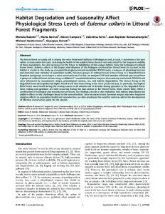
Fig. 1. Local maps and example study sites. (a) LANDSAT image of the counties of Essex and Suffolk, UK (51° 43’ 52” N, 0° 44’ 22” E to 51° 58’ 45” N, 1° 16’ 15” E), outlining the estuaries from which the 9 marshes were sampled. (b) An example of an Atriplex-dominated salt marsh at Shotley, Suffolk, on the Orwell estuary, ~2 km from the container port of Felixstowe. (c) LANDSAT image of the Wakatobi Marine National Park, SE Sulawesi, Indonesia (5° 28’ 24” S, 123° 42’ 00” E to 5° 32’ 45” S, 123° 52’ 30” E), illustrating the 4 main island regions of the park. Ten mangroves were sampled in 2 areas of the Kaledupa subregion of the park: North Kaledupa & Hoga Island (1) and Darawa Island (2). (d) An example of a small coastal Rhizophora mangrove forest at West Loho, Darawa Island

the Essex salt marshes, Green et al. 2009). Salt marsh fish were sampled from intertidal marsh creeks using 2 mm mesh (3 mm stretched) block nets placed at the mouth of randomly selected creeks at high tide; fish were caught in the nets as the creek drained on the ebb tide. Seasonal effects were reduced to a minimum through the intensive sampling over the 2 mo period. The maximum tidal range of the region was ~4.5 m; sampling was only performed when the tidal range was > 3.4 m. Mangrove sampling was performed during June to August 2008, during the Wakatobi dry season that lasts 6 to 8 mo of the year (Crabbe & Smith 2005). Mangrove fish were counted using a snorkelling visual census method (adapted from Nagelkerken et al. 2000), with 8 transects (50 × 3 m; area of 150 m2) established along a haphazardly selected part of the edge of the root stock for each mangrove. The maximum tidal amplitude in the Wakatobi MNP is 2.3 m,

and transect sampling was performed when the tide height was 1.9 ± 0.2 m above chart datum (Unsworth et al. 2007a). The sampled mangrove and salt marsh sites drained completely at low tide, exposing the adjacent intertidal mudflats (for salt marsh) or seagrass beds (for mangrove). All sampling was performed during daylight (07:00−17:00 h), and the repeated sampling of individual marshes and mangroves was spread across the 2 mo sampling periods. Each mangrove patch was sampled 8 times on separate high tides (although 2 to 3 mangrove patches were sampled on the same tide). Salt marshes often had 2 unconnected creeks in opposite areas of the marsh sampled on the same tide, in order to complete the sampling programme in the 2 mo seasonal window. A single salt marsh was sampled per tide. A different area of mangrove or marsh creek was sampled on each occasion, except for small habitat patches (e.g. Komo mangrove, at


181

Table 1. Definitions and codes of environmental and spatial variables that were measured: (a) 20 variables that were comparable between salt marsh (SM) and mangrove (M) habitats (coded A−T, see Figs. 3 & 4 and Tables 2 & S2), (b) 17 variables for salt marsh sites only (used in models A1 and A2), (c) 8 variables for mangrove sites only (used in models B1 and B2). The superscript in the variable column indicates if the variable was measured in situ (a), remotely (b), or both (ab: this was always remotely for salt marshes, in situ for mangroves). SM/M = salt marsh or mangrove; DW = dry weight Code Variable

Definition

(a) Comparable variables A Focal Patch Area (m2)ab

B C D E

F G

H I J K L M N O P

Q

R

S T

Area of the intertidal SM/M focal patch, with the landward boundary being marked by the seawall or coral cliff or limit of intertidal zone. Patches were defined as ‘separate’ when a subtidal channel completely divided the 2 patches from seaward to landward edge. Measured using satellite imagery. Focal Patch Perimeter of the intertidal SM/M focal patch, measured using GPS and satellite Perimeter (m)ab imagery. Seaward Edge Length of the seaward edge of the focal patch. Expanses of water < 50 m in Length (m)ab width had a straight line drawn across them (i.e. mouths of small marsh creeks). Maximum distance of a straight line between the seaward and landward edges of a Patch Depth (m)ab < 50 m in focal patch, measured perpendicular to the seaward edge. Shape Index (SI)ab Index of patch shape (Forman & Godron 1986), SI = P/√(πA), where P = length of focal patch perimeter, A = focal patch area. If SI = 1, patch is circular, if SI > 4, patch deviates significantly from circularity, e.g. by becoming increasingly elongate. Habitat (Halophyte) Percentage of the focal patch area covered by salt marsh plants or mangrove trees Cover (%)a (not including seagrass). The unvegetated part would be creeks or mud basins within. Percentage of the focal patch that is completely unvegetated (not covered by mangrove Unvegetated Area (%)a trees, halophytes or seagrass), or the percentage of the salt marsh that is dissected by creeks, i.e. the area occupied by creeks. Focal Patch Isolation Shortest distance from the centre of the primary creek of the SM/M focal patch to the (m)b edge of the nearest SM/M patch (nearest neighbour distance) Number of Patches Number of individual SM/M patches crossed by or within a circle of 500 m radius, within 500 mb centred from the mouth of the primary first-order creek of the focal patch. Number of Patches Number of individual SM/M patches crossed by or within a circle of 1 km radius, within 1 kmb centred from the mouth of the primary first-order creek of the focal patch. Area of Salt Marsh / Man- Total area of SM/M patches (including the focal patch) within a circle of 500 m radius, grove within 500 m (m2)ab centred from the mouth of the primary first-order creek of the focal patch. Area of Salt Marsh / Man- Total area of SM/M patches (including the focal patch) within a circle of 500 m radius, grove within 1 km (m2)ab centred from the mouth of the primary first-order creek of the focal patch. Length of Seaward Edge Length of seaward edge of SM/M patches (including the focal patch) within a circle within 500 m (m)ab of 500 m radius from the mouth of the primary first-order creek of the focal patch. Length of Seaward Edge Length of seaward edge of SM/M patches (including the focal patch) within a circle of within 1 km (m)ab 1 km radius from the mouth of the primary first-order creek of the focal patch. Distance to Adjacent Shortest distance to the subtidal channel (SM) or seagrass bed (M) from the edge of Habitats (m)ab the focal patch. Distance to ‘Open Sea’ Shortest distance to the estuary mouth (SM) or reef crest (M) from the edge of the (estuary mouth/reef focal patch. flat) (m)ab Sediment Organic For SM: the organic content (measured as ash-free dry weight of sediment) of 2 cm Content (g g−1)a deep sediment cores taken from bottom of marsh creek. For M: the total organic carbon (TOC; units g C g−1) content (from 6 minicores of 3 cm depth), measured with a TOC Analyzer after total inorganic carbon acidification with 2M HCl. Intertidal Area Measure of intertidal area quality. For SM: proportion of a semicircle of 200 m radius, Cover (%)ab centred from the mouth of the primary marsh creek that is intertidal mudflat (marked by mean low water springs), compared to subtidal waters. For M, mean percentage seagrass cover (estimated by eye) of 15 quadrats (1 m2) placed in the centre (core) of the seagrass bed adjacent to the mangrove focal patch. Water Temperature (°C)a Mean site daytime high tide water temperature of mangroves, sample-specific, daily high tide water temperature of sampled salt marsh creeks. Region/Estuary Region of sampled patch, a quality measure. SM: Colne, Blackwater, Orwell or Stour. M: Darawa or North Kaledupa. (Table 1 continued on next page)

Mar Ecol Prog Ser 466: 177–192, 2012

182

Table 1 (continued)

Code Variable

Definition

(b) Other salt marsh variables 1 Creek Area (m2)a 2 Creek Perimeter (m)a 3 4

5

6 7 8

9

10 11 12 13 14 15 16 17

Area of each SM creek sampled (upstream from the block net, by tracking GPS) at a site. Perimeter of each SM creek sampled (upstream from the block net, by tracking GPS) at a site. Perimeter:Area Ratio (m2)a Ratio between the SM creek perimeter (2) and area (1). Intertidal Area within Proportion of a semicircle of 500 m radius, centred from the mouth of the primary SM creek, that is intertidal mudflat (marked by mean low water springs), compared to 500 m (%)b subtidal waters. Intertidal Area within Proportion of a semicircle of 1 km radius, centred from the mouth of the primary SM 1 km (%)b creek, that is intertidal mudflat (marked by mean low water springs), compared to subtidal waters. Nearest Neighbour Distance to the nearest SM primary creek mouth from the SM focal patch in the Downstream (m)b downstream direction. Nearest Neighbour Distance to the nearest SM primary creek mouth from the SM focal patch in the upstream direction. Upstream (m)b Number of Individual Number of individual marshes crossed by or within a circle of 2 km radius, centred from Marshes within 2 km the mouth of the primary first-order creek of the SM focal patch. of Marshb Nereis Biomass (g m−2)a Mean DW of the polychaete Nereis diversicolor for an individual SM. Sampled from 24 sediment cores per marsh (3 cores per creek sampled; core area = 83.32 cm2, depth = 10 cm). Macoma Biomass (g m−2)a Mean DW of Macoma balthica for an individual SM. Measured as above. Hydrobia Biomass Mean DW of Hydrobia ulvae for an individual SM. Measured as above. (g m−2)a Corophium Biomass Mean DW of Corophium volutator for an individual SM. Measured as above. (g m−2)a Oligochaete Biomass Mean DW of Oligochaeta for an individual SM. Measured as above. (g m−2)a Tide Height (m)b High tide water height above chart datum (measured from Harwich) on the day of sampling. Salinity of water at 1 m depth taken at high tide at the position of the block net in the Salinitya SM creek measured using a refractometer. Dissolved Oxygen Mean dissolved oxygen of water at 1 m depth at the position of the block net in the SM (ml O2 l−1)a creek, measured using modified Winkler titration. Total Suspended Solids Total suspended solids of high tide water from creek mouth (1 m depth; DW of suspended solids from 1 l after filtration through a Whatman GF/F glass fibre filter). (g l−1)a

(c) Other mangrove variables 1 Rhizophora spp. Cover (%)a 2 3

4 5 6

7 8

Sonneratia spp. Cover (%)a Total Basal Area (TBA; m2 roots m−2)a

Prop Root Density (roots m−2)a Interdispersed Seagrass (%)a Edge Seagrass Cover (%)a Edge Seagrass Height (m)a Core Seagrass Height (m)a

Mean percentage cover of Rhizophora spp. prop roots along a 50 × 4 m line transect through the seaward 30 m of a mangrove focal patch. Number of transects depended on mangrove size, and ranged from 1 to 9. Mean percentage cover of Sonneratia spp. pneumatophore roots along a 50 × 4 m line transect through the seaward 30 m of a mangrove focal patch. Total area of a 1 m2 quadrat of mangrove-covered intertidal area occupied by pneumatophore and prop roots, calculated by the formula TBA = n [π(C/2π)2], where n is number of roots m−2 and C is mean circumference of 15 random roots in the quadrat, measured 30 cm above sediment. Roots were assumed to be circular. Mean number of Rhizophora prop roots m−2, counted 30 cm above sediment. Mean percentage cover of seagrass species along a 50 × 4 m line transect through the front 30 m fringe of a mangrove focal patch. Mean percentage seagrass cover (estimated by eye) of 15 quadrats (1 m2) placed in the fringing 10 m of the seagrass bed adjacent to the mangrove focal patch. Core seagrass cover is represented by variable R. Mean seagrass blade height of 15 quadrats (1 m2) placed in the fringing 10 m of the seagrass bed adjacent to the mangrove focal patch. Mean percentage seagrass cover (estimated by eye) of 15 quadrats (1 m2) placed in the fringing 10 m of the seagrass bed adjacent to the mangrove focal patch.


495 m2), where a marsh creek or mangrove edge was sampled more than once. For both habitats, fish density was expressed as ind. 100 m−2 (of transect or creek area), whilst species richness was expressed as species sample−1.

Statistical analysis To identify whether there were significant differences in fish community structure between sample sites, the fish species density data were square-root transformed and converted to a Bray-Curtis similarity table, from which an analysis of similarity (ANOSIM) test (PRIMER 6) was performed for each habitat (Clarke & Gorley 2006). To determine relationships between the measured environmental variables and fish species richness and density, a 2-step partial least squares (PLS) regression approach (Wold et al. 1984) was used, using the XL-STAT software with PLS add-on (Addinsoft). PLS is a regression that uses latent variables to identify linear and polynomial relationships between a set of predictor variables (x) and response variables (y) (Wold et al. 2001, Godhe & McQuoid 2003). PLS is effective when the number of predictor variables is higher than the number of observations, and when the predictor variables are highly correlated (strong multicollinearity; Carrascal et al. 2009). All variables and responses were log10(x+1) transformed and normalised before analysis to attempt to achieve symmetrical distributions (Wold et al. 2001). PLS analyses models are significant when the global goodness of fit statistic, Q2(cum) is greater than 0.0975. Relevant predictor variables can then be identified from their variable influence on the projection (VIP) score. First, individual PLS models for salt marsh fish species richness (A1), population density (A2), mangrove fish species richness (B1) and population density (B2) were run using all 37 salt marsh or 28 mangrove predictor variables (Table 2). For each of these models, a 2-step approach was used. An initial screening PLS analysis (PLS1) was run for each model, after which predictor variables with a VIP score of 1.0 were considered highly influential predictors for the model. Environmental variables with a VIP of 0.8 to 1.0 were considered moderately influential. Below 0.8, the variable was disregarded (Wold et al. 2001).

183

In order to observe general differences between the 2 habitats, the 4 PLS models were re-run using only 20 predictor variables comparable between salt marsh and mangrove habitats (models C1 to C4, Table 1). The VIPs of the 20 comparable predictor variables for salt marshes and mangroves were determined from PLS1, and were rank scored for each habitat, allowing direct comparison between mangroves and salt marshes of the relative importance of the predictor variables. PLS2 was also run with the PLS1 variables with a VIP > 1.0 to identify the highest influencing variables in the model. All PLS models from the analysis were significant at both the PLS1 and PLS2 stages, where Q2(cum) > 0.0975 for k model components (Table 3; Wold et al. 2001).

RESULTS Inter-habitat variability of fish assemblages English salt marshes within a close geographical proximity had significantly different fish population density, species richness and assemblage structure (mean values ± SE). A total of 2867 fish and 13 species were caught in the 9 salt marshes sampled. The overall salt marsh fish density was 4.95 ± 1.37 ind. 100 m−2 and ranged between samples from 0.59 ± 2.2 to 18.83 ± 9.24 ind. 100 m−2. Overall species richness was 2.25 ± 0.21 species sample−1 (0.33 ± 0.04 species 100 m−2), and ranged from 0 to 8 species sample−1. The 3 most abundant species in the salt marshes were the sea bass Dicentrarchus labrax (density of 2.56 ± 1.20 ind. 100 m−2), the goby Pomatoschistus microps (0.95 ± 0.25 ind. 100 m−2) and the atherinid Atherina presbyter (0.65 ± 0.32 ind. 100 m−2; Table S1). D. labrax represented 58.1% of all fish caught. Despite all the marshes being within 60 km of coastline, there were significantly different fish species assemblages across the 9 marshes sampled (ANOSIM Global R = 0.23, p < 0.001). The 4 sites with the lowest fish density and species richness (Fig. 2) all had similar species assemblages (Fig. S1 in the supplement at www.int-res. com/articles/suppl/m466p177_supp.pdf). Variations in the abundance of the 3 dominant fish species were responsible for the highest percentage of dissimilarity between sites (Table S1). As expected, Indonesian mangroves had higher fish population densities and species richness than UK salt marshes, with a total of 10 661 ind. from 64 species sampled. The overall density and richness was 111.51 ± 13.60 ind. 100 m−2 and 8.13 ± 0.49 species sample−1 (5.42 ± 0.32 species 100 m−2), but

184

Mar Ecol Prog Ser 466: 177–192, 2012

Fig. 2. Fish species richness and population density (n = 8 samples site−1; means ± SE) of UK salt marsh and Indonesian mangrove fish assemblages. The codes A1 to B2 refer to the associated partial least squares (PLS) regression models (Table 3). The colours of each bar designate the estuary (for salt marshes) or region of Kaledupa (for mangroves) in which the site was located (corresponding to variable T, Table 1). Note that the fish communities were sampled using underwater visual census in mangroves, and using block nets in salt marsh creeks

these had wide range between individual mangroves within a close geographic proximity. The smallest, but highly connected mangrove, Komo (area of 495 m2, 9 mangrove patches within 1 km radius), had the highest mean fish population density (298.39 ± 42.69 ind. 100 m−2) and richness (14.00 ± 0.71 species sample−1). The most isolated and sparsely vegetated mangrove, Furake (5.53 km from the nearest mangrove), had the lowest fish population density (2.27 ± 0.66 ind. 100 m−2) and the lowest species richness (1.63 ± 0.38 species sample−1; Table 2). All mangrove sites had significantly different fish assemblages, apart from Lamohasi and Kaluku (ANOSIM Global R = 0.58, p < 0.01), with the 3 most abundant fish species responsible for the highest percentage of dissimilarity between sites (Fig. S1). The 3 most abundant mangrove fish species were the shoaling atherinid Atherinomorus lacunosus (mean density of 46.25 ± 10.2 ind. 100 m−2, 41.5% of all fish sampled), the cardinalfish Sphaeramia orbicularis (21.16 ± 3.6 ind. 100 m−2) and an unidentified shoaling anchovy species, family Engraulidae (13.86 ± 5.4 ind. 100 m−2).

Key drivers of fish population density and species richness The PLS analyses demonstrated that mangrove and salt marsh fish assemblages were influenced by different spatial variables. Predictor variables had a high or low influence within the PLS model, as determined by the VIP score (Fig. 3, Table S2), with the influence resulting in a positive or negative correlation with the response variable (fish species richness or population density). Termed the ‘Intertidal Area’, the proportion of intertidal mudflat (compared to subtidal) within a 200 m radius around the salt marsh was the variable that scored the highest VIP, and had the strongest negative influence over salt marsh fish species richness (PLS model A1, Fig. 3; untransformed correlation r = −0.559, VIP = 1.494 ± 0.16). Further influential variables (VIP > 1.0) included the Shape Index, Creek Area and the Perimeter:Area Ratio of a marsh creek. There was a strong influence of Daily Water Temperature on fish population density (PLS model A2; r = 0.456, VIP = 1.537 ± 0.36). Also influential (VIP > 1.0) were the Shape Index, the

1 2 3 4 5 6 7 8 9 10 11 12 13 14 15 16 17

S T

P Q R

A B C D E F G H I J K L M N O 533583 4836 1838 666 2.04 61.74 39.50 1141 0.3 1.7 233030 480092 1544 2443 256

12.72 –

865 356 0.51 72.27 63.24 1356 1865 4.0 4.75 1.27 3.66 0.01 0.03 3.78 33.17 5.44 0.08

Individual Marsh Area (m2) Marsh Perimeter (m) Marsh Seaward Edge (m) Marsh Depth (m) Shape Index (no unit) Habitat Cover (%) Unvegetated Area (%) Patch Isolation (m) Patches within 500 m of Marsh Patches within 1 km of Marsh Area of Salt Marsh w/n 500 m (m2) Area of Salt Marsh w/n 1 km (m2) Seaward Edge w/n 500 m (m) Seaward Edge w/n 1 km (m) Distance to Adjacent Habitat (subtidal channel) (m) Distance to Open Sea (estuary mouth) (m) Sediment Organic Content (AFDW; g g−1) Intertidal Area Cover (intertidal mudflat w/n 200 m radius) (%) Water Temperature (°C) Estuary (qualitative variable)

Other salt marsh variables Creek Area (m2) Creek Perimeter (m) Creek Perimeter:Area Ratio Intertidal Area cover w/n 500 m (%) Intertidal Area cover w/n 1 km (%) Distance to NN Downstream (m) Distance to NN Upstream (m) Patches within 2 km of marsh Nereis Biomass (g m−2) Macoma Biomass (g m−2) Hydrobia Biomass (g m−2) Corophium Biomass (g m−2) Oligochaete Biomass (g m−2) Tide Height (m) Salinity Dissolved Oxygen (ml O2 l−1) Total Suspended Solids (g l−1)

6029 0.098 90.29

Mean

Comparable salt marsh variables

91 53 0.16 36.56 23.97 138 468 2.0 0.00 0.00 0.00 0.00 0.00 3.50 27.00 3.11 0.04

7.00 –

2990 0.075 57.78

53415 1308 588 140 1.26 28.46 4.36 138 0.0 0.0 53415 53415 588 663 35

Min

2510 1010 1.55 100.00 100.00 2930 3355 8.0 26.43 15.92 99.37 0.17 0.29 4.10 24.50 8.99 0.14

22.00 –

9820 0.119 100.00

2038000 12763 3426 1498 2.52 95.64 71.50 2930 1.0 4.0 533831 804814 2383 4350 890

Max

1 2 3 4 5 6 7 8

S T

P Q R

A B C D E F G H I J K L M N O

Mean

Other mangrove variables Rhizophora Cover (%) Sonneratia Cover (%) Total Basal Area (m2 roots m−2) Prop Root Density (roots m−2) Interdispersed Seagrass (%) Edge Seagrass Cover (%) Edge Seagrass Height (cm) Core Seagrass Height (cm)

60.05 7.08 0.41 44.58 7.94 25.36 27.23 36.61

Individual Mangrove Area (m2) 76970 Mangrove Perimeter (m) 1126 Mangrove Seaward Edge (m) 381 Mangrove Depth (m) 143 Shape Index (no unit) 4.02 Habitat Cover (%) 44.58 Unvegetated Area (%) 22.10 Patch Isolation (m) 787 Patches within 500 m of Mangrove 2.0 Patches within 1 km of Mangrove 5.2 Area of Mangrove w/n 500 m (m2) 78756 Area of Mangrove w/n 1 km (m2) 147337 Seaward Edge w/n 500 m (m) 558 Seaward Edge w/n 1 km (m) 1019 Distance to Adjacent Habitat 24 (seagrass bed) (m) Distance to Open Sea (reef flat) (m) 1379 Sediment Total Organic Carbon (g C g−1) 0.119 Intertidal Area Cover (adjacent 47.82 7.00 seagrass bed core cover) (%) Water Temperature (°C) 27.21 Region (qualitative variable) –

Comparable mangrove variables

6.41 0.00 0.16 1.25 0.00 4.80 9.44 7.32

25.96 –

440 0.063 88.88

495 108 24 15 2.61 1.25 0.00 50 0.0 0.0 3143 3143 44 44 3

Min

93.65 38.2 0.65 83.00 62.12 53.53 49.78 65.20

27.80 –

2860 0.337

648000 4460 1800 550 7.91 93.65 66.90 5530 5.0 10.0 360633 614460 1299 1798 124

Max

Table 2. Mean, minimum and maximum values for the 37 salt marsh and 28 mangrove variables (defined in Table 1), including the 20 variables comparable between habitats (A−T; see Fig. 4). w/n: within, AFDW: ash-free dry weight, NN: nearest neighbour

Green et al.: Differential spatial effects on coastal habitats 185

186

Mar Ecol Prog Ser 466: 177–192, 2012

Fig. 3. Top 6 influencing environmental variables (variable importance of the projection, VIP ± SD) for salt marsh and mangrove fish species richness (models A1 and B1) and population density (A2 and B2) after the second stage of partial least squares (PLS) regression, PLS2. All 36 salt marsh and all 29 mangrove environmental variables were used in the corresponding models. Variables are considered strongly (VIP > 1.0), moderately (1.0 > VIP > 0.8; between the dashed lines) or not influential (VIP < 0.8) over the model. The letters and numbers before the variable names refer to the codes in Tables 1 & 2 and Fig. 4. Symbols (+ or –) associated with the bars indicate the direction of correlation of that variable with the relevant predictor variable, either species richness or density. Q2(cum) is the proportion of the total variation of the response (y) variable that can be predicted by k components, and was significant for all models (Q2(cum) > 0.0975). For model A1, ‘Estuary’ is a qualitative variable, indicating that there are estuary-specific differences between salt marsh species richness. P:A = Perimeter:Area, SE: Seaward Edge, TSS: Total Suspended Solids, w/n: within

length of the seaward edge and the depth of the salt marsh (Fig. 3, Table S2) The variables with the highest influence on the models, with a VIP > 1.0, are shown in Fig. 3. The number of individual mangrove patches within 1 km of the focal patch was the spatial variable with the highest VIP and strongest positive influence over mangrove fish species richness (PLS model B1, untransformed correlation r = 0.486, VIP = 1.234 ± 0.08). Mangrove habitat complexity was also important (VIP > 1.0), with 2 variables (Total Basal Area, Prop Root Density) having positive correlations with

species richness. In contrast, Prop Root Density was the variable with the highest VIP and a strong positive influence over fish population density (PLS model B2, log-transformed r = 0.598, VIP = 1.209 ± 0.06). Rhizophora Forest Cover, Shape Index and the Length of Mangrove Seaward Edge within 500 m radius of the mangrove site all had a VIP > 1.0, and were considered highly influential over fish population density (Fig. 3, Table S2). PLS regression models C1 to C4 utilised the 20 comparable environmental variables that were applicable for both salt marshes and mangroves (Table 1).


187

Table 3. Models fitting the partial least squares (PLS) regression of environmental predictor variables, x, against the response variable of either species richness (species sample−1) or density (ind. 100 m−2), after the second step of the PLS (PLS2). Models A1 and A2 use all 37 variables measured for salt marshes, models B1 and B2 use all 28 variables measured for mangroves (see Table 1). Models C1 to C4 used the 20 variables comparable between mangrove and salt marsh habitats (see Table 1). k: number of components in the model; Q2(cum): proportion of the total variation of the response (y) variable that is predicted by k components; R2x (cum): proportion of the sum of squares of all the predictor (x) variables explained by k components; R2y(cum): proportion of the sum of squares of the response variable explained by k components; R2(model): goodness of fit of the resultant regression equation to the data Model A1 A2 B1 B2 C1 C2 C3 C4

Habitat

Response

Variables

k

Q2(cum)

R2x(cum)

R2y(cum)

R2(model)

Salt marsh Salt marsh Mangrove Mangrove Salt marsh Salt marsh Mangrove Mangrove

Richness Density Richness Density Richness Density Richness Density

37 37 28 28 20 20 20 20

2 2 3 3 1 2 3 3

0.385 0.405 0.509 0.611 0.294 0.397 0.558 0.587

0.251 0.600 0.847 0.791 0.399 0.663 0.873 0.855

0.452 0.505 0.614 0.631 0.332 0.492 0.644 0.655

0.452 0.505 0.661 0.684 0.332 0.492 0.682 0.721

For both fish species richness and population density, the rank scores of these 20 variables after PLS1 were compared between the 2 habitats (Fig. 4). Whereas for mangrove fish species richness, the Shape Index (variable E), Patch Isolation (variable H), Number of Patches within 1 km (variable J) and Area of Patches within 1 km (variable L) were considered highly influential (VIP > 1.0 after PLS2), in salt marsh habitats only Shape Index (variable E) and Adjacent Intertidal Area Cover (variable R) were highly influential (Fig. 4a). For fish density in mangroves, Shape Index, Patch Isolation, Number of Patches within 1 km and Number of Patches within 500 m (vari-

Fig. 4. Comparison of scored importance of 20 comparable environmental predictor variables defined by (a) species richness (partial least squares, PLS, models C1 and C3) and (b) population density (PLS models C2 and C4) of mangrove and salt marsh fish communities after 1 PLS regression (PLS1). Variables are coded with letters, defined in Table 1. Variables are rank scored from 1 (least influential) to 20 (most influential) through the variable importance of the projection (VIP) result of the PLS1. Variables that scored higher than the dashed lines s–s (for salt marsh variables) or m–m (for mangrove variables) and are coloured blue have a VIP > 1.0 in the second PLS regression (PLS2) and can be classed as strongly influential over the model. Those coloured black have a VIP of 0.8 to 1.0 in PLS2, and are classed as moderately influential over the model. The diagonal dashed lines indicate x = y ± 25% CI. Variables that fall on this line can be considered equally influential in both mangrove and salt marsh habitats. (c) Symbols (+ or −) associated with the letters indicate the direction of correlation of that variable with the relevant predictor variable, either species richness or population density. Symbols above the letter refer to salt marsh responses, symbols to the left refer to mangrove responses. Symbols are only present for predictor variables whose VIP after PLS1 is > 1.0

able I) were the highly influential variables, compared to Shape Index, Patch Depth (variable D) and Water Temperature (variable S) for salt marshes (Fig. 4).

Mar Ecol Prog Ser 466: 177–192, 2012

188

Shape Index (variable E), was the only variable that influenced fish species richness and population density in both habitats to the same extent. As the shape index increased, i.e. the circular habitat patch deviated from circularity, e.g. by increasing elongation, both fish density and species richness decreased in both salt marshes and mangroves. In addition to Shape Index, mangrove fish density and richness were strongly influenced by 2 connectivity-related variables: Patch Isolation (variable H), and Number of Mangroves within 1 km (variable J). Neither of these measures of connectivity was influential in the salt marshes. For salt marshes but not mangroves, other influential variables were the Adjacent Intertidal Area Cover (variable R and Marsh Estuary/ Mangrove Region, variable T). With respect to salt marsh fish population density, influential variables were Water Temperature, Shape Index, Patch Depth and Patch Seaward Edge Length (variables S, E, D and C), with the latter 2 variables demonstrating negative relationships with fish density. None of these variables was influential in determining fish population density for mangroves. Two variables were found to have opposite influences on fish species richness between salt marsh and mangrove. Habitat Cover (variable F), a measure of patch complexity, was found to have a positive influence for the salt marsh species richness but a negative influence for the mangroves (Fig. 4a), whereas the Area of Salt Marsh or Mangrove within 1 km radius of the patch (variable L), a measure of connectivity, had a negative influence for salt marsh species richness, but a positive influence for mangroves.

DISCUSSION Key drivers of assemblage structure Whilst mangroves and salt marshes both provide increased food, shelter and nursery function to fish, there appear to be different spatial variables that influence fish assemblage richness and density in these 2 habitat types. Salt marsh fish species richness and density were strongly influenced by both structural connectivity (Adjacent Intertidal Area Cover) and patch structural complexity variables (Shape Index, Length of Seaward Edge; Fig. 3). A larger area of mudflat adjacent to a salt marsh reduced fish species richness. Such a relationship has not been previously identified in salt marshes, and suggests that the presence of a large intertidal mudflat between salt marshes and the subtidal estuarine channel reduces

the connectivity of that salt marsh with other nearby habitat types (Table 2). Jelbart et al. (2007) identified a similar relationship, with a negative correlation between the species richness of mangrove fish that migrate into seagrass beds, and the distance between these 2 habitats. It may be that extensive mudflats provide sufficient feeding opportunities for juvenile fish, given that these species feed on invertebrates common in both salt marsh creeks and mudflats (Green et al. 2009, 2012), thereby reducing the dispersion of fish on each tide. The increased shelter provided by the presence of eelgrass Zostera sp. on an adjacent mudflat may also increase fish abundance in salt marsh habitats (Irlandi & Crawford 1997). However, intertidal eelgrass is very scarce around the eastern coast of England (UK Environment Agency unpublished data), and so was not measured as a predictor variable and assumed to have little impact on the results of this study. Although fish have previously been shown to feed preferentially in salt marshes after swimming over extensive (>1 km) mudflats (Laffaille et al. 2001, 2002), our results suggest that the importance of particular marshes as feeding sites depends on the local geomorphology of that particular length of coastline (Allen et al. 2007). We found that patch Shape Index (variable E) was important in both salt marsh and mangrove habitats (Fig. 4). As the shape of a habitat patch deviates from circularity (e.g. by becoming increasingly elongate), the core area of high-quality habitat decreases, which, in mangroves and salt marshes, increases the proportion of mangrove fringe or fragmented edge habitat available (Forman & Godron 1986, Saunders et al. 1991). However, an increase in available edge in other coastal habitats such as seagrass can result in a higher fish abundance and richness (Boström et al. 2011), but a negative correlation was observed to mangrove edge variables, such as focal patch perimeter, in this study (Fig. 3). This may be due to the poor refuge quality provided by fragmented, low root density, mangrove edge habitat, which results in a higher predation risk to fish (Sheaves 2005, Verweij et al. 2006). Mangrove fish species richness and density were influenced by a mixture of structural connectivity and habitat complexity-based variables. Mangrove sites with the highest fish species richness and population density had a highly complex root network and high mangrove habitat cover and were well connected with adjacent mangroves within a 1 km radius. In contrast, the temperate salt marsh creek− intertidal mudflat−subtidal channel continuum is less


structurally complex and provides little 3-dimensional shelter compared to a complex mangrove root system (Möller et al. 1999, West & Zedler 2000, Gratwicke & Speight 2005). According to Hutchinson (1953), low complexity landscapes with fewer niches will result in fewer habitat specialists. Only 1 fish species (the common goby Pomatoschistus microps) could be considered a habitat specialist in the European salt marsh, with the other fish species found in salt marshes also present in the adjacent sublittoral habitats (Mathieson et al. 2000, Cattrijsse & Hampel 2006). In contrast, the tropical coastal seascape has many specialist fish species associated with individual patch types along the topographically complex mangrove−seagrass−reef continuum (Gratwicke & Speight 2005, Wilson et al. 2008). Verweij et al. (2006) reported that a complex root structure in mangroves reduces predation pressure, whilst high mangrove habitat cover will provide increased shade. This attracts mangrove-specific fish species that are not found in the equally structurally complex but unshaded adjacent seagrass beds, such as the highly abundant cardinalfish Sphaeramia orbicularis. The high density of roots in a complex mangrove will primarily attract juvenile fish (Laegdsgaard & Johnson 2001).

Between-habitat differences of spatial drivers Intertidal mangroves are situated in a highly heterogeneous coastal seascape, with a range of environmental conditions and habitat structures from the mangroves and seagrasses with high shelter and food availability, to the increased competition and limited resource availability in the adjacent coral reef flats (Ricklefs 1987, Ebeling & Hixon 1991, Gratwicke & Speight 2005, Verweij et al. 2006, Bouillon et al. 2007, Unsworth et al. 2008). As a result, fish utilise a highly connected system requiring a mosaic of closely-linked mangrove patches to maintain high density and species richness, as shown by the strong influence of the connectivity variables in our study (Fig. 4, Table S2). The importance of a mosaic of habitats has been previously highlighted (Franklin & Prugh et al. 2008, Franklin & Lindenmayer 2009), but as we have shown (Fig. 3), the structural properties of the adjacent patches in the mosaic will also strongly influence community structure (Tanner 2006). Our study also showed that the arrangement of the surrounding patches of mangrove was more significant than the presence of adjacent seagrass and reef patch on mangrove fish species richness and density

189

(Fig. 3, Table S2). This differs from previous studies on Indo-Pacific seagrass beds and reefs, which demonstrated that the presence of a mangrove patch significantly altered the fish assemblages of the adjacent patch type (Dorenbosch et al. 2004, 2005, Jelbart et al. 2007, Unsworth et al. 2008). Our result may reflect the general high density of seagrass found in the Wakatobi MNP and shorter distances between mangrove fringe and adjacent seagrass beds compared to other studies identifying mangrove−seagrass proximity as a factor in structuring assemblages (Dorenbosch et al. 2004, Jelbart et al. 2007). However, studies by Pittman et al. (2004) and Meynecke et al. (2008) identified that the spatial configuration of Australian mangrove patches (using connectivity indices, e.g. mean nearest neighbour) had strong positive correlations with fish and prawn assemblage density and landings. This supports the strong positive correlation between the number of mangrove patches within 1 km radial extent of the focal mangrove and fish population density observed in this study (Fig. 3). Complex seascapes may also result in direct connectivity, reducing fish movement paths between patches (Hitt et al. 2011). Despite the numerous studies demonstrating the importance of the habitat mosaic (Ricketts 2001, Tanner 2006, Prugh et al. 2008, Franklin & Lindenmayer 2009), and its strong influence over fish communities in mangrove habitats, the mosaic’s relative importance was not as important in salt marshes (Fig. 4). Conversely to mangroves, temperate salt marsh creeks exist in a more topographically homogenous coastal seascape (West & Zedler 2000). The temperate coastal seascape has a lower fish diversity than the tropical one (Roy et al. 1998), therefore the low interspecific competition and low functional redundancy between fish species drives a localised community (Tilman 1994). Such a community may have a low reliance on a network of interlinked salt marsh patches, contrary to mangroves. In support of this, we have recently shown high levels of site fidelity in juvenile and adult fish species in this mosaic of European salt marshes (Green et al. 2012). Whilst the current study characterises sites through fish distribution, it can be easily replicated to incorporate species groups that utilise other habitats, through integration of other environmental variables into the model (Moilanen et al. 2005, Nagelkerken et al. 2008). It should be noted, however, that the influential variables reported for the species richness and density of the overall assemblage may not be the same influential variables that control the abundance of an individual species of fish.

190

Mar Ecol Prog Ser 466: 177–192, 2012

There are strong seasonal patterns in the use of salt structure into reserve design and conservation marshes by larval and juvenile fish as feeding and (Borthagaray et al. 2009, Gladstone 2009). Our findnursery grounds, with peaks during the early sumings have identified that fish population density and mer months (Laffaille et al. 2000, Green et al. 2009). species richness in salt marshes and mangroves are The current study was undertaken at the time of year driven by different spatial variables. Within Europe, when fish species richness and abundance was highwhere the Water Framework Directive has set statuest, which is consistent with the greatest use of tory minimum targets for the maintenance of both marshes by fish. In Indo-Pacific mangroves, fish spesalt marsh area and function and coastal fish divercies richness peaks during the wet season due to sity (Best et al. 2007), studies such as this could help high juvenile recruitment, but fish biomass and popsupport the design of successful conservation strateulation density may show no seasonal variation (Ikegies by providing the spatial configuration paramejima et al. 2003). This study was undertaken during ters for the creation of optimum salt marsh habitat for the dry season in the Wakatobi, therefore identifying fish communities or particular species. In Indonesia, patterns of fish utilisation that are representative of coastal management is decentralised and occurs on a 6 to 8 mo of the year (Crabbe & Smith 2005). Consecommunity-based scale (Siry 2011). As a result, the quently, while there may be times during the growth implementation of a small (500 m wide) communitycycle of different species when our findings do not led no-take zone (NTZ) over the reef crest and flat apply, the sampling periods chosen represent periods around Hoga Island, Wakatobi MNP, was successful of high fish habitat use. and acceptable to local fishers, although mangroves This study has important implications for future were not part of the NTZ (Unsworth et al. 2007b, management of coastal systems, including other Clifton & Unsworth 2010). The results of this study intertidal habitat continuums, such as estuarine mansupport the designation of small mangrove patches, grove−mudflat systems. The coastline of northwest such as those around the Darawa area of the WakaEurope, in particular, has been heavily modified for tobi MNP (e.g. Loho or Lamohasi, Figs. 1 & 2) as hundreds of years, resulting in the loss of seagrass NTZs to benefit local fisheries without taking valubeds, biogenic reefs and other coastal habitats able fishing grounds away from local stakeholders. (Airoldi & Beck 2007). With increasing threats to salt Therefore, differing approaches to management marsh and mangrove habitats from coastal erosion, need to be taken for each habitat in order to conserve climate change and reclamation (van der Wal & Pye the fish biodiversity of the coastal seascape. 2004, Primavera 2005, Alongi 2008), our study has Acknowledgements. We thank Operation Wallacea, the demonstrated that if the aim of conservation is to staff at Hoga Island Marine Centre and the Ministry of maximise fish density and species richness, then Research and Technology, Indonesia, who provided a habitat protection has to occur on an individual focal research permit for D.J.S. We also thank the Essex Wildlife patch for salt marshes, and across the larger seascape Trust and other landowners for access to marshes in the UK. for mangroves (Fig. 3). Our results have some impliThe comments of 4 anonymous reviewers aided the revision of this manuscript. This project was supported by a Natural cations for the SLOSS debate, with a higher species Environment Research Council funded PhD studentship richness and population density of fish that utilise awarded to B.C.G. (Award Code NER/S/A/2006/14133). mangroves in a network of smaller patches, whilst single salt marshes with a suitable shape and close to LITERATURE CITED a subtidal channel adequately support their associated fish communities. Often attempts at defining Aburto-Oropeza O, Ezcurra E, Danemann G, Valdez V, optimal reserve design have focused on the spe- ➤ Murray J, Sala E (2008) Mangroves in the Gulf of Califorcies−area relationship, but such a debate may be nia increase fishery yields. Proc Natl Acad Sci USA 105: 10456−10459 inadequate for designing marine reserves, particuAdams AJ, Ebersole JP (2009) Mechanisms affecting recruitlarly for salt marshes and mangroves, where few fish ment patterns of fish and decapods in tropical coastal species are permanent inhabitants, but show tidal, ecosystems. In: Nagelkerken I (ed) Ecological connectivtemporal and ontogenetic patterns of use (Neigel ity among tropical coastal ecosystems. Springer, Heidel2003, Sheaves et al. 2006, Green et al. 2009). Future berg, p 185–228 Airoldi L, Beck MW (2007) Loss, status and trends for coastal research should focus on the connectivity of fish marine habitats of Europe. Oceanogr Mar Biol Annu Rev between salt marshes and the estuarine subtidal 45:345−405 channels. ➤ Allen DM, Haertal-Borer SS, Milan BJ, Bushek D, Dame RF Our study supports the importance of integrating (2007) Geomorphological determinants of nekton use of intertidal salt marsh creeks. Mar Ecol Prog Ser 329:57−71 connectivity between patches and individual patch


191

➤ Alongi DM (2008) Mangrove forests: resilience, protection ➤ Faunce CH, Serafy JE (2008) Selective use of mangrove ➤

➤ ➤

➤ ➤

➤ ➤

➤

➤ ➤

➤

➤

➤

➤

from tsunamis and responses to global climate change. Estuar Coast Shelf Sci 76:1−13 Beck MW, Heck KL, Able KW, Childers DL and others (2001) The identification, conservation and management of estuarine and marine nurseries for fish and invertebrates. Bioscience 51:633−641 Best M, Massey A, Prior A (2007) Developing a saltmarsh classification tool for the European water framework directive. Mar Pollut Bull 55:205−214 Borthagaray AI, Brazeiro A, Giménez L (2009) Connectivity and patch area in a coastal marine landscape: disentangling their influence on local species richness and composition. Aust Ecol 34:641−652 Boström C, Pittman SJ, Simenstad C, Kneib RT (2011) Seascape ecology of coastal biogenic habitats: advances, gaps, and challenges. Mar Ecol Prog Ser 427:191−217 Bouillon S, Dehairs F, Velimirov B, Abril G, Vieira Borges A (2007) Dynamics of organic and inorganic carbon across contiguous mangrove and seagrass systems (Gazi Bay, Kenya). J Geophys Res 112:G02018 Carrascal LM, Galván I, Gordo O (2009) Partial least squares regression as an alternative to current regression methods used in ecology. Oikos 118:681−690 Cattrijsse A, Hampel H (2006) European intertidal marshes: a review of their habitat functioning and value for aquatic organisms. Mar Ecol Prog Ser 324:293−307 Clarke KR, Gorley RN (2006) Primer v6: user manual. Primer-E, Plymouth Clifton J, Unsworth RKF (2010) Future directions for marine conservation in the Coral Triangle. In: Clifton J, Unsworth RKF, Smith DJ (eds) Marine conservation and research in the Coral Triangle: the Wakatobi National Park. Nova Publishers, New York, NY, p 251–258 Cocheret de la Morinière E, Pollux BJA, Nagelkerken I, Hemminga MA, Huiskes AHL, van der Velde G (2003) Ontogenetic dietary changes of coral reef fishes in the mangrove-seagrass-reef continuum: stable isotopes and gut-content analysis. Mar Ecol Prog Ser 246:279−289 Costanza R, D’Arge R, de Groot R, Farber S and others (1997) The value of the world’s ecosystem services and natural capital. Nature 387:253−260 Crabbe MJC, Smith DJ (2005) Sediment impacts on the growth rates of Acropora and Porites corals from the fringing reefs of Sulawesi, Indonesia. Coral Reefs 24: 437−441 Das S, Vincent JR (2009) Mangroves protected villages and reduced death toll during Indian super cyclone. Proc Natl Acad Sci USA 106:7357−7360 Dorenbosch M, van Riel MC, Nagelkerken I, van der Velde G (2004) The relationship of reef fish densities to the proximity of mangrove and seagrass nurseries. Estuar Coast Shelf Sci 60:37–48 Dorenbosch M, Grol MGG, Christianen MJA, Nagelkerken I, van der Velde G (2005) Indo-Pacific seagrass beds and mangroves contribute to fish density and diversity on adjacent coral reefs. Mar Ecol Prog Ser 302:63−76 Ebeling AW, Hixon MA (1991) Tropical and temperate reef fishes: a comparison of community structures. In: Sale PF (ed) The ecology of fishes on coral reefs. Academic Press, San Diego, CA, p 509–563 Fahrig L (2003) Effects of habitat fragmentation on biodiversity. Annu Rev Ecol Evol Syst 34:487−515 Faunce CH, Serafy JE (2006) Mangroves as fish habitat: 50 years of field studies. Mar Ecol Prog Ser 318:1−18

➤

➤

➤

➤

➤

➤ ➤

➤ ➤

➤

➤

➤ ➤ ➤

shorelines by snappers, grunts, and great barracuda. Mar Ecol Prog Ser 356:153−162 Forman RTT, Godron M (1986) Landscape ecology. Wiley, New York, NY Franklin JF, Lindenmayer DB (2009) Importance of matrix habitats in maintaining biological diversity. Proc Natl Acad Sci USA 106:349−350 Gladstone W (2009) Conservation and management of tropical coastal ecosystems. In: Nagelkerken I (ed) Ecological connectivity among tropical coastal ecosystems. Springer, Heidelberg, p 565–606 Godhe A, McQuoid MR (2003) Influence of benthic and pelagic environmental factors on the distribution of dinoflagellate cysts in surface sediments along the Swedish west coast. Aquat Microb Ecol 32:185−201 Gratwicke B, Speight MR (2005) The relationship between fish species richness, abundance and habitat complexity in a range of shallow tropical marine habitats. J Fish Biol 66:650−667 Green BC, Smith DJ, Earley SE, Hepburn LJ, Underwood GJC (2009) Seasonal changes in community and trophic structure of fish populations of five salt marshes along the Essex coastline, United Kingdom. Estuar Coast Shelf Sci 85:247−256 Green BC, Smith DJ, Grey J, Underwood GJC (2012) High site fidelity and low site connectivity of temperate salt marsh fish populations: a stable isotope approach. Oecologia 168:245−255 Grober-Dunsmore R, Frazer TK, Beets JP, Lindberg WJ, Zwick P, Funicelli NA (2008) Influence of landscape structure on reef fish assemblages. Landscape Ecol 23(Suppl 1):37−53 Gustafson EJ, Gardner RH (1996) The effect of landscape heterogeneity on the probability of patch colonization. Ecology 77:94−107 Harborne AR, Mumby PJ, Micheli F, Perry CT, Dahlgren CP, Holmes KE, Brumbaugh DR (2006) The functional value of Caribbean coral reef, seagrass and mangrove habitats to ecosystem processes. Adv Mar Biol 50:57−189 Hewitt JE, Thrush SF, Halliday J, Duffy C (2005) The importance of small-scale habitat structure for maintaining beta diversity. Ecology 86:1619−1626 Hitt S, Pittman SJ, Nemeth RS (2011) Diel movements of fishes linked to benthic seascape structure in a Caribbean coral reef ecosystem. Mar Ecol Prog Ser 427: 275−291 Hutchison GE (1953) The concept of pattern in ecology. Proc Acad Nat Sci Philadelphia 105:1−12 Ikejima K, Tongnunui P, Medej T, Taniuchi T (2003) Juvenile and small fish in a mangrove estuary in Trang province, Thailand: seasonal and habitat differences. Estuar Coast Shelf Sci 56:447−457 Irlandi EA, Crawford MK (1997) Habitat linkages: the effect of intertidal salt marshes and adjacent subtidal habitats on abundance, movement and growth of an estuarine fish. Oecologia 110:222−230 Jelbart JE, Ross PM, Connolly RM (2007) Fish assemblages in seagrass beds are influenced by the proximity of mangrove forests. Mar Biol 150:993−1002 Laegdsgaard P, Johnson C (2001) Why do juvenile fish utilise mangrove habitats? J Exp Mar Biol Ecol 257: 229−253 Laffaille P, Feunteun E, Lefeuvre JC (2000) Composition of fish communities in a European macrotidal salt marsh

192

➤

➤

➤

➤

➤

➤

➤

➤

➤

➤ ➤

➤ ➤

➤ ➤ ➤

➤ ➤

Mar Ecol Prog Ser 466: 177–192, 2012

(the Mont Saint-Michel Bay, France). Estuar Coast Shelf Sci 51:429−438 Laffaille P, Lefeuvre JC, Schricke MT, Feuntein E (2001) Feeding ecology of 0-group sea bass, Dicentrarchus labrax, in salt marshes of Mont Saint Michel Bay (France). Estuaries 24:116−125 Laffaille P, Feunteun E, Lefebvre C, Radureau A, Sagan G, Lefeuvre JC (2002) Can thin-lipped mullet directly exploit the primary and detritic production of European macrotidal salt marshes? Estuar Coast Shelf Sci 54: 729−736 Layman CA, Quattrochi JP, Peyer CM, Allgeier JE (2007) Niche width collapse in a resilient top predator following ecosystem fragmentation. Ecol Lett 10:937−944 Little C (2000) The biology of soft shores and estuaries. Oxford University Press, Oxford Mathieson S, Cattrijsse A, Costa MJ, Drake P, Elliot M, Gardner J, Marchand J (2000) Fish assemblages of European tidal marshes: a comparison based on species, families and functional guilds. Mar Ecol Prog Ser 204: 225−242 Meynecke JO, Lee SY, Duke NC (2008) Linking spatial metrics and fish catch reveals the importance of coastal wetland connectivity to inshore fisheries in Queensland, Australia. Biol Conserv 141:981−996 Moilanen A, Franco AMA, Early RI, Fox R, Wintle B, Thomas CD (2005) Prioritizing multiple-use landscapes for conservation: methods for large multi-species planning problems. Proc R Soc Lond B Biol Sci 272:1885−1891 Möller I, Spencer T, French JR, Leggett DJ, Dixon M (1999) Wave transformation over salt marshes: a field and numerical modeling study from north Norfolk, England. Estuar Coast Shelf Sci 49:411−426 Mumby PJ, Edwards AJ, Arias-González JE, Lindeman KC and others (2004) Mangroves enhance the biomass of coral reef fish communities in the Caribbean. Nature 427:533−536 Nagelkerken I, Dorenbosch M, Veberk WCEP, Cocheret de la Morinière E, van der Velde G (2000) Importance of shallow water biotopes of a Caribbean bay for juvenile coral reef fishes: patterns in biotope association, community structure and spatial distribution. Mar Ecol Prog Ser 202:175−192 Nagelkerken I, Blaber SJM, Bouillon S, Green P and others (2008) The habitat function of mangroves for terrestrial and marine fauna: a review. Aquat Bot 89:155−185 Neigel JE (2003) Species-area relationships and marine conservation. Ecol Appl 13:138−145 Pittman SJ, McAlpine CA, Pittman KM (2004) Linking fish and prawns to their environment: a hierarchical landscape approach. Mar Ecol Prog Ser 283:233−254 Pittman SJ, Caldow C, Hile SD, Monaco ME (2007) Using seascape types to explain the spatial patterns of fish in the mangroves of SW Puerto Rico. Mar Ecol Prog Ser 348: 273−284 Primavera JH (2005) Mangroves, fishponds and the quest for sustainability. Science 310:57−59 Prugh LR (2009) An evaluation of patch connectivity measures. Ecol Appl 19:1300−1310 Prugh LR, Hodges KE, Sinclair RE, Brashares JS (2008) Effect of habitat area and isolation on fragmented animal populations. Proc Natl Acad Sci USA 105:20770−20775 Ricketts TH (2001) The matrix matters: effective isolation in fragmented landscapes. Am Nat 158:87−99 Ricklefs RE (1987) Community diversity: relative roles of Editorial responsibility: Ivan Nagelkerken, Nijmegen, Netherlands

local and regional processes. Science 235:167−171

➤ Roy K, Jablonski D, Valentine JW, Rosenberg G (1998) Mar➤ ➤ ➤ ➤ ➤

➤ ➤ ➤ ➤

➤

➤

➤ ➤

➤

➤ ➤

➤

ine latitudinal diversity gradients: tests of causal hypotheses. Proc Natl Acad Sci USA 95:3699−3702 Saunders DA, Hobbs RJ, Margules CR (1991) Biological consequences of ecosystem fragmentation: a review. Conserv Biol 5:18−32 Sheaves M (2005) Nature and consequences of biological connectivity in mangrove systems. Mar Ecol Prog Ser 302:293−305 Sheaves M, Baker R, Johnston R (2006) Marine nurseries and effective juvenile habitats: an alternative view. Mar Ecol Prog Ser 318:303−306 Siry HY (2011) In search of appropriate approaches to coastal zone management in Indonesia. Ocean Coast Manag 54:469−477 Skilleter GA, Olds A, Longergan NR, Zharikov Y (2005) The value of patches of intertidal seagrass to prawns depends on their proximity to mangroves. Mar Biol 147: 353−365 Tanner JE (2006) Landscape ecology of interactions between seagrass and mobile epifauna: the matrix matters. Estuar Coast Shelf Sci 68:404−412 Tilman D (1994) Competition and biodiversity in spatially structured habitats. Ecology 75:2−16 Tjørve E (2010) How to resolve the SLOSS debate: lessons from species diversity models. J Theor Biol 264:604−612 Unsworth RKF, Wylie E, Bell JJ, Smith DJ (2007a) Diel trophic structuring of seagrass bed fish assemblages in the Wakatobi Marine National Park, Indonesia. Estuar Coast Shelf Sci 72:81−88 Unsworth RKF, Powell A, Hukom F, Smith DJ (2007b) The ecology of Indo-Pacific grouper (Serranidae) species and the effect of a small-scale no take area on grouper assemblage, abundance and size frequency distribution. Mar Biol 152:243−254 Unsworth RKF, Salinas de Leon P, Garrard SL, Jompa J, Smith DJ, Bell JJ (2008) High connectivity of Indo-Pacific seagrass fish assemblages with mangrove and coral reef habitats. Mar Ecol Prog Ser 353:213−224 Van der Wal D, Pye K (2004) Patterns, rates and possible causes of saltmarsh erosion in the Greater Thames area (UK). Geomorphology 61:373−391 Verweij MC, Nagelkerken I, de Graff D, Peeters M, Bakker EJ, van der Velde G (2006) Structure, food and shade attract juvenile coral reef fish to mangrove and seagrass habitats: a field experiment. Mar Ecol Prog Ser 306: 257−268 Wedding LM, Lepczyk CA, Pittman SJ, Friedlander AM, Jorgensen S (2011) Quantifying seascape structure: extending terrestrial spatial pattern metrics to the marine realm. Mar Ecol Prog Ser 427:219−232 West JM, Zedler JB (2000) Marsh−creek connectivity: fish use of a tidal salt marsh in Southern California. Estuaries 23:699−710 Wilson SK, Burgess SC, Cheal AJ, Emslie M and others (2008) Habitat utilization by coral reef fish: implications for specialists vs. generalists in a changing environment. J Anim Ecol 77:220−228 Wold S, Albano C, Dunn WJ, Edlund U and others (1984) Multivariate data analysis in chemistry. In: Kowalski BR (ed) Chemometrics — mathematics and statistics in chemistry. Reidel, Dordecht, p 17–95 Wold S, Sjöström M, Eriksson L (2001) PLS-regression: a basic tool of chemometrics. Chemom Intell Lab Syst 58:109−130 Submitted: July 4, 2011; Accepted: May 2, 2012 Proofs received from author(s): September 25, 2012