Halfmoon – A new Paradigm for Complex Network Visualization∗ Ignacio Alvarez-Hamelin†, Marco Gaertler‡, Robert G¨orke‡ and Dorothea Wagner‡
Abstract We propose a new layout paradigm for drawing a nested decomposition of a large network. The visualization supports the recognition of abstract features of the decomposition, while drawing all elements. In order to support the visual analysis that focuses on the dependencies of the individual parts of the decomposition, we use an annulus as the general underlying shape. This method has been evaluated using real world data and offers surprising readability.
1
Introduction
Current research activities in computer science and physics aim at understanding large and complex networks like the physical Internet, the World Wide Web, or peer-to-peer systems. The design of adequate visualization methods for such networks is an important step towards this aim. As these networks are large or even huge on one hand, and evolving on the other hand, customized visualizations concentrating on their intrinsic structural characteristics are required. The (implicit) relevance of nodes is the most commonly investigated feature. It is usually expressed by a nested decomposition of the node set. Common visualizations of such large networks usually suffer a trade-off between the details of visually shown elements and the visible amount of represented information. In this paper we propose a layout method that has properties of abstract visualizations while showing all nodes and edges. The technique works in two phases. In the first, abstract phase, the nested decomposition determines the general shape of the layout. This step compares to general abstract visualization techniques. In the second phase, the individual nodes and edges are placed. This stage is parameterized to offer a scalable trade-off between the overall quality and the required computational effort. Many applications are especially interested in the inter-shell edges of the decomposition. Thus we employ a partial annulus as the underlying shape, since it offers a large area ∗ The authors gratefully acknowledge financial support from the European Commission within FET Open Projects COSIN (IST-2001-33555) and DELIS (contract no. 001907) and the DFG under grant WA 654/13-3. † Universit´ e Paris Sud, Laboratoire de Physique Th´ eorique 91405 Orsay CEDEX, France.
[email protected] ‡ Universit¨ at Karlsruhe (TH), Informatics, ITI Wagner, 76128 Karlsruhe, Germany. {gaertler,rgoerke,dwagner}@informatik.uni-karlsruhe.de
1
for uniformly drawing these edges. At the same time, however, it supports an individual handling of the shells. Several layout techniques have been developed driven by the ambitious goal to properly visualize the Autonomous System network. One important approach is the landscape metaphor [3]. Introduced by Baur et.al., it modifies a conventional layout technique by a framework of underlying constraints that are based on analytic properties. The global shape of the network is induced by the position of structurally important elements, which automatically conceals inferior parts. Thus, it reflects the ‘landscape’ of importance, either in two or three dimensions. LaNet-vi [1] is another approach that uses analytic properties to define a suitable global shape, which in this case consists of concentric rings. It then tries to fit the whole network accordingly, while the overall readability is achieved by showing only a small sample of the edge set. The method we present in the following also utilizes analytic properties to define a suitable global shape, however, it eliminates the requirement of sampling the edges and further enhances human perception of analytic properties. Although the idea of initially determining the global shape via analytic properities is borrowed from LaNet-vi, our technique is more flexible and its results are more readable. This paper is organized as follows. After giving some notation, we present our new layout paradigm in Section 2. An empirical study, using real world examples of the physical Internet and collaboration networks, is given in Section 3. Finally, we conclude the paper in Section 4 with a brief summary.
2
Layout Method
In this section, we present our new layout paradigm and offer some suggestions on sophisticated node placement.
2.1
Nested Decomposition
Before describing our visualization paradigm, we give some notation. Let G = (V, E) be an undirected graph and H = (V =: V0 ) V1 ) · · · ) Vk ) Vk+1 := ∅) a nested decomposition of V . The height of H is k and the height of a node v is defined as i such that v ∈ Vi \ Vi+1 . The set Vi is also called the i-th layer of H and its node-induced subgraph is denoted by G(Vi ). The k-th layer is called top layer. The i-th shell Si is defined as the set Vi \ Vi+1 and contains all nodes with height i.
2.2
Layout Paradigm
Visualizations of large networks, i. e., those with more than 10,000 nodes or edges, usually suffer a trade-off between the details of visually shown elements and the amount of represented information. For example, drawing all nodes and edges can lead to crowded layouts, while restricting to groups of nodes or edges is generally accompanied by loss of information. These are extreme examples and should both be avoided. Our goal is the visualization of all nodes and edges in addition to revealing the characteristics of the given hierarchical decomposition. More precisely, we focus on properties like the size of shells and the connectivity within or between shells.
2
Abstracted visualizations of the hierarchical decomposition offer the best readability of the abovementioned properties. However such techniques only preserve most information in case of uniform distributions of these properties. In the case where most values are overshadowed by some maximum value, many interesting details will be suppressed. For example, if the edge count between shells is distributed in a power-law like fashion, then connections between shells that have a very small edge count will not be visible. Such a situation is depicted in Figure 1, where many edges (between shells) have a very little edge count compared to the maximum edge count. 1
2
17 16 15 14 13 12 11 10
3
4
5
6
7
8
9
Figure 1: Abstracted version of the AS graph (May 1st, 2001). The area of the nodes is proportional to the number of nodes having that height. The thickness of the super-edges is proportional to their edge count. Super-edges with too little edge count are omitted. We overcome this issue by using the layout of the abstracted graph as a blueprint but still draw all elements. The shapes and positions of the shells are determined by selected properties and define the reserved drawing area for the contained nodes. Inter-shell edges will be drawn as straight lines and intra-shell edges may be drawn with bends.
2.3
Implementation of the Layout Paradigm
We propose as a general underlying shape of the visualization an annulus. The shells are lined up along a predefined angular range, placing the bottom and the top shell at the extremes. Thus, the shells correspond to annular segments. User-defined properties then determine the individual dimensions of these segments. In order to increase readability, small gaps that separate neighboring segments can be included. Placing the individual nodes is by far the most computationally demanding task. Simple strategies such as random placement offer an easy recognition of the shells’ shapes. On the other hand, more sophis-
3
ticated techniques can additionally reveal the internal structure of the shells while requiring more time and storage. The general setup has the following parameters (also shown in Figure 2): inner radius (rmin ), outer radius (rmax ) and total angle (ω) of the annular segment. These parameters define the available drawing area. For each shell, there is an individual inner radius (ri ), an outer radius (Ri ) and an angle (αi ). Thus,
A0i
Ri
Ai ri
ω αi rmin
rmax
Figure 2: General parameter setup for the annulus paradigm. the segment of each shell is divided into two parts (Ai and A0i ) that are used to draw the nodes and the intra-shell edges, respectively. The dimensions of the parameters ri , Ri and αi are determined by user-defined properties which can be the number of nodes per shell, the number of intra-shell edges, the degree of connectivity, etc. Optionally, the size of one of the parts can be set to zero, in order to focus on specific properties of the other part. Especially, for large networks, the focus is typically on the nodes.
2.4
Suggestions for Sophisticated Node Placement
There are several ways to layout the interior of the annular segments in a more sophisticated way. Typical approaches rely on force-directed methods. In the simplest cases, adjacent nodes attract each other while non-adjacent nodes repel each other. Due to the general shape imposed by our layout paradigm, the forces should be scaled differently for intra-shell and inter-shell edges. By uprating intra-shell edges, the node placement within a segment reflects the internal structure. Another issue to consider are the hard boundaries of the annular segments. Soft and hard clipping can prevent nodes from clamping onto these
4
boundaries due to a blend of inter-shell attractions and intra-shell repulsions. The preferable type of clipping heavily depends on the input graph. As a common side-effect of these forces, the available drawing area of the annular segments might not be fully exploited. Conventional gravitational forces are only suitable if the shape of the corresponding segment is approximately a square. In all other cases, direction-dependent scaling, multiple centers of gravity or even partially repulsive forces are recommended, in order to spread out nodes. A minor drawback of these techniques are their implementational demands. Moreover, the proper choice of the coordinate system strongly depends on the selection of forces, i. e., boundary checking that is part of clipping is achieved best using spherical coordinates, while attraction and repulsion favor cartesian coordinates due to the simple computation of distances. Further issues are the proper choice of the involved parameters for the forces.
3
Results
In this section, we present the visualizations we obtained with our layout paradigm for various large networks. In the first part of our experimental study, we focus on the Autonomous System graph and its core hierarchy, while in the second part, we examine collaboration networks. Our visualizations are obtained using the following setup: ω = π, rmax /rmin = 4, αi ∝ f (|Vi |), ri ∝ g(|Ei |), and Ri = 0, where Vi is the set of nodes in the i-th shell, Ei is the set of intra-shell edges of the i-th shell, and f, g are nonnegative, monotonically increasing functions, like square-root or logarithm, used for scaling.
3.1
Autonomous System Graph
An Autonomous System (AS) is a collection of computer devices that route Internet traffic and belong to the same administrative authority. The resulting network consists of nodes representing each operating AS and of edges connecting to two ASes, if they have a traffic exchange agreement, which is established via the Border Gateway Protocol (BGP). Standard data sets that represent the network between 2001 and 2005 contain 10,000-20,000 nodes and 23,000-41,000 edges. With respect to importance, the AS network can be decomposed into several parts, i. e., backbone, national, regional, and local providers as well as customers. However, such a partition is ambiguous and hard to extract. We use the concept of k-cores ([6, 2]) that have already been used for similar analyses [5, 4]. It is related to the degree of a node, but substantially differs from a decomposition based purely on degree. Table 1 shows the layouts using different scalings for radius and angle. Obviously, proportions are well readable using linear functions, while the interaction between shells is clearly obtainable using logarithmic functions f for scaling the angles. In fact, the simultaneous representation of several scaling combinations offers the identification of different aspects at the same time. Although the shell sizes heavily differ, only a square-root scaling function g for the outer radius is suitable in the case of the Autonomous System network. A
5
g(|Ei |) – outer radius sqrt
log
sqrt log
f (|Vi |) – angle
linear
linear
Table 1: Visualizations of the AS (1st March, 2005) using different scaling options. logarithmic function g could be applied if only the general tendency of the shell sizes is important. In particular, we obtain the following facts from the matrix-like representation: First, more than 75% of all nodes are contained in the 1-, 2-, or 3-shell (linear-linear view). Second, 2-, 3-shell as well as the top shell have the largest density with respect to intra-shell edges (log-linear view). Third, the sizes of the shells’ intra-shell edge sets (between 2-shell and top shell) are not monotonically decreasing (log-log view). Fourth, most of the inter-shell edges connect either the 1-, the 2-, or the 3-shell with the top shell (log-sqrt view). Moreover, many other inter-shell edges connect to the top shell. Finally, there are also nontop shells that have (relatively) many inter-shell edges connecting them with low-level shells. Summarizing, many interesting and useful properties of the decomposition can be extracted from the matrix view at a glance. The above list is only a brief example. Depending on user-defined goals, a small selection of views can be sufficient to emphasize the required properties.
3.2
Collaboration Networks
Collaboration networks are usually extracted from large publication databases. In these networks nodes commonly correspond to actors and edges connect two actors that have a common publication. We use the database DBLP1 which is a freely available and well maintained collection of computer science publications. Since dense subgraphs correspond to heavily collaborating groups of actors, the collaboration networks are also decomposed using the k-core concept ([6, 2]). Table 2 shows the layouts using different scalings for radius and angle. The network consists of the heads of different sites of a EU projects as well as their direct collaborators. In contrast to the AS network, the edges are not mainly distributed between the low cores and the core. 1 http://www.informatik.uni-trier.de/~ley/db/
6
g(|Ei |) – outer radius sqrt
log
sqrt log
f (|Vi |) – angle
linear
linear
Table 2: Visualizations of the collaboration network within DELIS (2005).
3.3
Internet Movie Data Base
For the final evaluation, we used the Internet Movie DataBase (IMDB). The database primarily contains the bipartite relation of movies and performing actors. It stores information about 1.3 million actors and movies and roughly 3.7 million relations. We used the IMDB network to evaluate the scalability of our algorithm. The asymptotic time complexity of both the k-core decomposition and the layout algorithm is linear. Indeed, our Java-based implementation calculated a layout in less then two minuites (excluding I/O-operations) using roughly 4.5 gigabyte of main memory. In contrast, the rendering process including the transparancy effects required six hours and 10 gigabyte of main memory on the same machine. The results are shown in Table 3. The presence of a 0-core (isolated nodes) is due to incomplete data.
4
Conclusion
We presented a new paradigm that has properties of an abstract visualization while showing all nodes and edges. We focused on characteristics of a given hierarchical decomposition. The general shape is an annulus and the individual shells of the decomposition are drawn within certain annular segments. The dimensions of these segments are defined by analytic properties. Due to the underlying abstract traits that are thus visualized, we achieve high readability of the decomposition, including interactions between shells and relative sizes of node or edge sets. An additional feature is the scalable trade-off between overall quality and required computational time. The fastest layouts still represent all key characteristics, while high quality visualizations reveal further information of the decomposition and the individual shells. Simultaneously visualizing the same networks using different scalings can offer complementary information. The paradigm has been evaluated using the Autonomous System graph and collaboration networks, using the k-cores as nested hierarchical decomposition. 7
g(|Ei |) – outer radius sqrt
sqrt log
f (|Vi |) – angle
linear
linear
Table 3: Visualizations of the IMDB (2003).
8
log
References [1] Jos´e Ignacio Alvarez-Hamelin, Luca Dall’Asta, Alain Barrat, and Alessandro Vespignani. k-core decomposition: A tool for the visualization of large scale networks. arXiv:cs.NI/0504107, 2005. [2] V. Batagelj and M. Zaverˇsnik. Generalized cores. Preprint 799, Universtiy of Ljibljana, 2002. [3] Michael Baur, Ulrik Brandes, Marco Gaertler, and Dorothea Wagner. Drawing the as graph in 2.5 dimensions. In Proceedings of the 12th International Symposium on Graph Drawing (GD’04), volume 3383 of Lecture Notes in Computer Science, pages 43–48, 2005. [4] Marco Gaertler and Maurizio Patrignani. Dynamic analysis of the autonomous system graph. In IPS 2004 – Inter-Domain Performance and Simulation, pages 13–24, March 2004. [5] Christos Gkantsidi, Milena Mihail, and Ellen Zegura. Spectral analysis of internet topologies. In IEEE Infocom 2003, 2003. [6] S. B. Seidman. Network structure and minimum degree. Social Networks, 5:269–287, 1983.
9